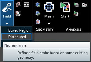
Distributed |
The distributed field probe samples selected surfaces or lines at regular spacing intervals. It is a powerful tool with inherent algorithms to process data and record the data in a useful and common format. Distributed field probes encompass and process data from many mesh nodes on a surface or along a line in the geometric model. The larger region of these probes better captures both peak and null features of electromagnetic fields, which could be missed when using data from a single node.
For calculating the electromagnetic fields and the transfer functions, EMA3D performs a 5 % running bandwidth average on the field data. Then, EMA3D performs a Fast Fourier Transform of each location and averages the raw values together. Finally, EMA3D then performs another pass and "smooths" them out by averaging neighboring frequencies together with a sliding window.
Click
 Field within the Probes section under the EMA3D tab in the ribbon. Then select Distributed from the drop-down menu.
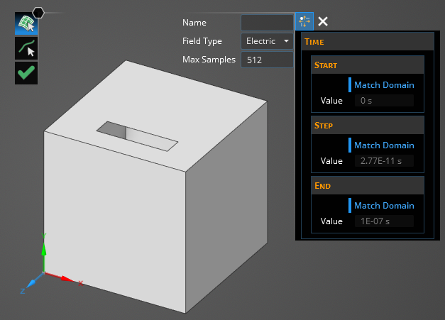
The default probe field type is Electric, suitable to measure the electric field within the distributed region. In order to measure the magnetic field, change the probe field type to Magnetic in the Properties panel. In the Properties panel, the time properties can also be adjusted.
Two options for setting the probe will also appear in the top left of the model window. Use the top, default option
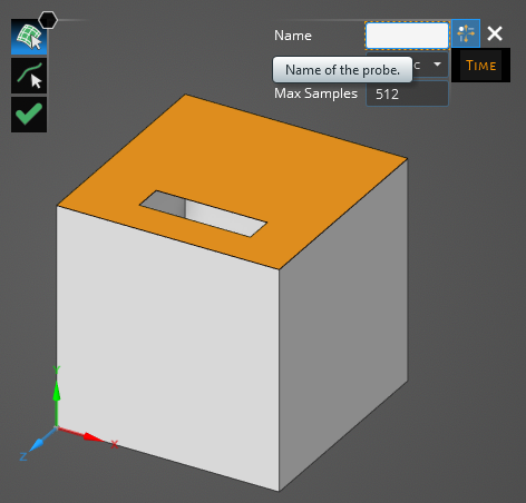
to define the boundaries of the distributed probe on a surface by selecting a surface in the model window or in the structure tree. Use the second tool to define the boundaries of the distributed probe on a line by selecting a line in the model window or in the structure tree. Note that only one surface or line can be selected per probe. The selected geometry will glow orange once selected and you will be redirected to name the probe (default naming convention is Field Probe #). Click OK
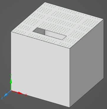
 to create the probe. A series of green points will appear indicating the lattice point locations (where probe measurements will be taken) included within the probe boundaries. For distributed probes, the software will automatically select points for you based on the geometry selected and the maximum number of sample points in order to cover the selected region at semi-regular intervals from boundary to boundary.
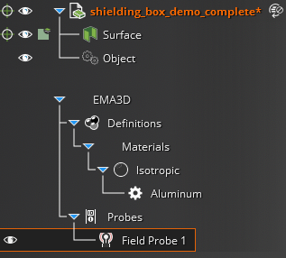
The probe should now be added to the Simulation Tree under the Probes node as Field Probe # or whichever name it was given.
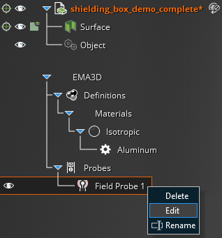
The probe can be edited at any time by right clicking it in the Simulation Tree and selecting Edit from the pop-up menu.
To visualize the Distributed Probe results, see here.
Entry | Meaning |
|---|---|
Name | Name of the probe. |
Field Type | The field quantity to measure. It can be set to Electric or Magnetic to measure the electric field or the magnetic field. |
Max Samples | Maximum number of locations to probe. |
Entry | Meaning |
|---|---|
Start: Match Domain | Match the start time to the FDTD domain. |
Start: Value | The time the probe starts recording data. The default start time matches the simulation start time. |
Step: Match Domain | To which domain to match the probe time step: Domain matches the probe time step to the FDTD domain time step. Frequency sets the probe time step such that it captures up to the highest supported frequency of the domain (this time step is coarser than the Domain time step and results in smaller files). False allows the user to set the probe time step manually. |
Step: Value | To which domain to match the probe time step:
|
End: Match Domain | Match the end time to the FDTD domain. |
End: Value | The number of time steps between probe data being written out (e.g., setting Skip to 2 will record every other time step). |
Other Resources
EMA3D – © 2026 EMA, Inc. Unauthorized use, distribution, or duplication is prohibited.