3D |
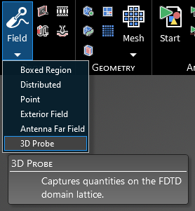
The 3D probe is a powerful tool that can be used to visualize electric field, magnetic field, electric current, or air conductivity on the FDTD domain lattice. It is similar to the animation probe, but the 3D probe allows users to visualize volumes and cut planes rather than surfaces.
Click
 Field within the Probes section under the EMA3D tab in the ribbon. Then select 3D from the drop-down menu.
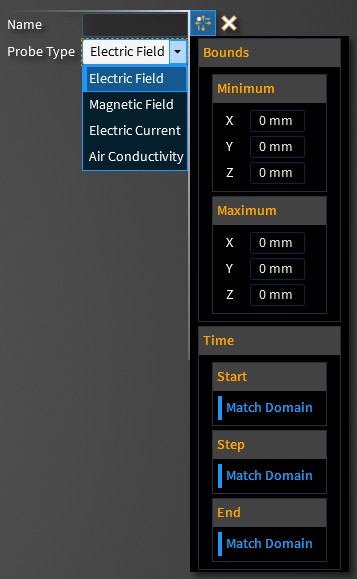
In the Properties Panel, adjust the probe field type and time properties as desired.
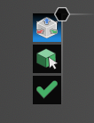
Two options for setting the probe will appear in the top left of the model window. The top, default option
 defines the integration boundaries of the field probe using a drag box with directional arrows. The second option
 defines the integration boundaries of the field probe based on a selected body.
Click OK
 to complete the probe definition. A series of green points will appear indicating the lattice point locations (where probe measurements will be taken) included within the probe boundaries.
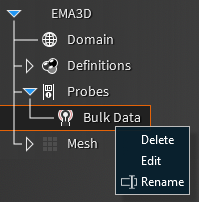
Adjust the definitions of the probe at any time by right clicking it within the Simulation Tree and selecting Edit from the pop-up menu.
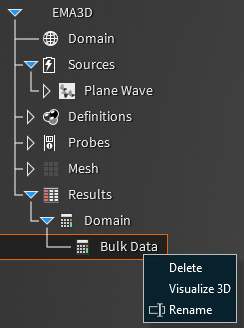
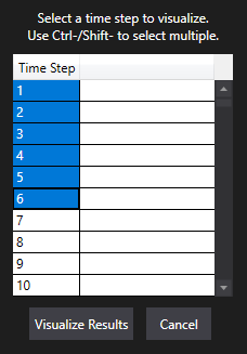
To visualize the 3D Probe results, right click the 3D Bulk Data probe within the Results node in the Simulation Tree and select Visualize 3D. Then select the time steps to visualize in the pop-up window.
In the bottom right corner of the model window, select the
 Contours button to view the contoured volume. Select the
 Cut Plane button to view a cut plane through the contoured volume.
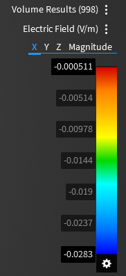
The contours, fields, and time step plotted can be adjusted in the Settings panel that appears at the right side of the model window.
Entry | Meaning |
|---|---|
Name | Name of the probe. |
Probe Type | Field quantity to probe. |
Entry | Meaning |
|---|---|
Min - X | Minimum x location of the probe. |
Min - Y | Minimum y location of the probe. |
Min - Z | Minimum z location of the probe. |
Min - X | Maximum x location of the probe. |
Min - Y | Maximum y location of the probe. |
Min - Z | Maximum z location of the probe. |
Entry | Meaning |
|---|---|
Start - Match Domain | Match the start time to the FDTD domain (blue = True). |
Start - Value | The probe start time. |
Step - Match Domain | To which domain to match the probe time step: Domain matches the probe time step to the FDTD domain time step. Frequency sets the probe time step such that it captures up to the highest supported frequency of the domain (this time step is coarser than the Domain time step and results in smaller files). False allows the user to set the probe time step manually. |
Step - Value | The probe time step. |
End - Match Domain | Match the end time to the FDTD domain (blue = True). |
End - Value | The probe end time. |
Entry | Meaning |
|---|---|
X | Down sampling X |
Y | Down sampling Y |
Z | Down sampling Z |
EMA3D – © 2026 EMA, Inc. Unauthorized use, distribution, or duplication is prohibited.