X vs T

The X vs T Probe Group type is so named because using probes in this category produces files with an X vs T format, where ‘X’ is a quantity and ‘T’ is time. There are eight different probe types associated with the X vs T Probe Group. These probe types are listed below:

Each of these probe types are discussed in separate subsections below.

There is only one keyword associated with the Screen Probe. This keyword is listed below.

The Screen Probe is a convenient feature that allows the user to write certain electromagnetic quantities to the computer screen (or to a log file) attached to the computer on which the EMA3D® program is executing. These quantities include:

Electric fields (x, y, or z components), Magnetic fields (x, y, or z components), Thin wire currents Cylindrical conductor currents MHARNESS cable bundle currents Thin gap voltages EMA3D Seam voltages

The output format of this probe is:

time, quantity1, quantity2, quantity3,…etc.

Since the Screen Probe results in information being written to the screen or monitor, or possibly to a log file, there is no defined output file generated.

The New Probe is a powerful tool with inherent algorithms to process data and record the data in a useful and common format. The New Probe involves the following electromagnetic quantities:

Electric fields (x, y, or z components), Magnetic fields (x, y, or z components), Thin wire currents and voltages Cylindrical conductor currents and voltages MHARNESS cable bundle currents and voltages Thin gap voltages Seam voltages Barrier article voltages

The powerful features of the New Probe include: Time domain calculations Frequency domain calculations Transfer function calculations Prony analysis

The frequency domain calculations are done during the computation so there is no need to store the corresponding time domain results unless desired. With the New Probe, one can easily specify a range or bandwidth of frequencies. In addition to frequency domain results, transfer functions (see below) can also be computed and written in the same easy format as that given above. If frequency domain information is specified, the associated time domain responses from which the frequency data is computed, should decay to a value close to zero to affect proper spectral analysis. Failure to adhere to this will compromise the spectral data

For calculating the electromagnetic fields and the transfer functions, EMA3D performs a 5 % running bandwidth average on the field data. Then, EMA3D performs a Fast Fourier Transform of each location and averages the raw values together. Finally, EMA3D then performs another pass and "smooths" them out by averaging neighboring frequencies together with a sliding window.

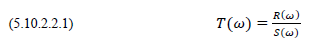
A transfer function, T(ω), is the ratio of a particular response, R(ω), to the driving source, S(ω), that produced the response. As indicated by the, “ω”, all waveforms are in the frequency domain. This relationship is given by Equation (5.10.2.2.1) below.

The response, R(ω), can be any of those listed above. The driving source, S(ω), is also any of those allowable within EMA3D. When using transfer functions, only one source waveform, S(ω), should be driving the model. That is, a plane wave source with no other nodal sources present, or perhaps a collection of nodal sources all utilizing the same source waveform. Multiple source waveforms will all contribute to the response, R(ω), thereby affecting the transfer function.

Inspection of Equation (5.10.2.2.1) shows a transfer function to be a normalized response. This eliminates the spectral character of the source. For example, if a plane wave source, with a particular electric field waveform, were used to drive a model, then the resultant response would be dependent upon the spectral character of the electric field waveform. Computing a transfer function would eliminate the spectral effects of the source producing a response as if CW plane waves, of 1.0 volt/meter amplitude across the band employed by the source, were driving the model.

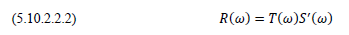
When a transfer function, T(ω), has been calculated for a particular response, R(ω), then the corresponding response, R’(ω), associated with another source, S’(ω), possessing the same geometric relationship to the geometry of the object, can be obtained using Equation (5.10.2.2.2) below.

A source with the same geometric relationship means the new source, S’(ω), must possess the same geometrical relationship and same configuration to the object being model. For example, the current channel must be identically placed or the plane wave must possess the same propagation vector and electric field polarization.

The ability to analytically curve fit a time domain result is available through the implementation of Prony analysis. Prony analysis provides an analytical representation of a time domain response waveform in terms of complex exponentials and amplitudes. The procedure identifies the complex frequency poles of a response and calculates the corresponding residues. The response is then just a summation of all residues multiplied by exponentially damped sinusoids, as defined by Equation (5.10.2.2.3) below.

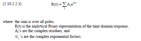
A Prony representation enables temporal extension beyond the range of the finite difference computational time limit and the calculation of frequency and transfer function results. The Prony analysis algorithm spans a large range of skip factors and orders selecting the best-fit pair. Although a large range of skip factors and orders are examined to provide the best fit, the result may not always be acceptable. The Prony time domain representation should be inspected before frequency domain results are accepted.

There are two keywords associated with the New Probe. These keywords are listed below.

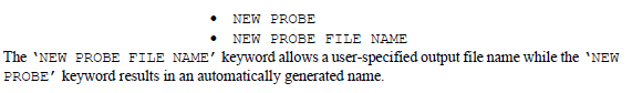
The use of the ‘New Probe’ keyword produces seven different automatically generated output file names depending upon what was specified. For any New Probe output, the characters, “npr”, are concatenated onto the end of the input file base name. These characters are designed to abbreviate the New Probe utility. The file extension of all New Probe output files is, “.dat”. Thus, if the input file name was, “Model1.emin”, then any New Probe specification will result in at least one file with the name:

“Model1npr**********.dat”

The asterisks stand for other characters yet to be explained. For the New Probe utility, a numerical result, a Prony result, or a combination of the two, can be specified. If a numerical result is designated, then the characters, “numer”, are concatenated onto the end of file base name, producing the result:

“Model1nprnumer*****.dat”

For a Prony result specification, the characters, “prony”, are concatenated onto the end of file base name, producing the result:

“Model1nprprony*****.dat”

With the New Probe utility, the option of specifying a time domain result, a frequency domain result, a transfer function result, or any combination of the three is available. If time domain information is specified, then the characters, “time”, are concatenated onto the end of the file base name producing the result:

“Model1nprnumertime*.dat” or “Model1nprpronytime*.dat”

If frequency domain information is specified, then the characters, “freq”, are concatenated onto the end of the file base name producing the result:

“Model1nprnumerfreq*.dat” or 153 “Model1nprpronyfreq*.dat”

If transfer function information is specified, then the characters, “tran”, are concatenated onto the end of the file base name producing the result:

“Model1nprnumertran*.dat” or “Model1nprpronytran*.dat”

With a Prony specification, an additional file is produced. This file contains the numerical result and the associated Prony analysis reproduction, within the same file for easy comparison. This file has the characters, “comp”, concatenated onto the end of the file base name producing the result:

Model1nprpronycomp*.dat”

The remaining asterisk is a place-holder for an integer that numbers the files. Each New Probe specification increments this number by one. Therefore, if one New Probe was specified, then depending upon the nature of the specification, files with the following names may be generated.

Model1nprnumertime1.dat Model1nprnumerfreq1.dat Model1nprnumertran1.dat Model1nprpronytime1.dat Model1nprpronyfreq1.dat Model1nprpronytran1.dat Model1nprpronycomp1.dat

If a second new probe is specified, then depending upon the nature of the specification, files with the following names may be generated.

Model1nprnumertime2.dat Model1nprnumerfreq2.dat Model1nprnumertran2.dat Model1nprpronytime2.dat Model1nprpronyfreq2.dat Model1nprpronytran2.dat Model1nprpronycomp2.dat

The information within a numerical time domain file (e.g. “Model1nprnumertime1.dat”) is provided in the following format, with the quantity order corresponding to the order of appearance in the EMA3D input file.

time, quantity1, quantity2, quantity3,…etc.

The information within a numerical frequency domain or transfer function file (e.g. “Model1nprnumerfreq1.dat” or “Model1nprnumertran1.dat”) is provided in the following format, with the order corresponding to the order of appearance in the EMA3D input file.

frequency, quantity1, quantity2, quantity3,…etc.

The information within the associated Prony analysis files, if specified, is identical to the numerical output file format described above. The information within the additional Prony analysis file (e.g. “Model1nprpronycomp1.dat”) is provided in the following form, with the order corresponding to the order of appearance in the EMA3D input file.

time, quantity1, Prony quantity1, quantity2, Prony quantity2, quantity3, Prony quantity3,…etc.

The Voltage Difference Probe allows the easy computation of voltages between two difference locations or points. With a few keywords and descriptors, many voltages can be computed between points or regions of points.

The integration path between any two points, programmed within the algorithms of EMA3D for voltage computations, is first along the x-coordinate direction, then along the y-coordinate direction, followed by the z-coordinate direction. Remember, the computation of voltages is path independent only for conservative electric fields (𝛁×𝑯 = 0.0).

Since the Voltage Difference Probe allows the specification of regions of points, the user should be aware of the potential generation of large quantities of data, if such are used. If voltage differences between two regions consisting of 10 x 10 x 10 cells are specified, then the output would consist of 1 million (10002) voltages for every output time record.

There are two keywords associated with the New Probe. These keywords are listed below.

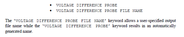
The use of the ‘Voltage Difference Probe’ keyword results in an automatically generated output file name. The automatically generated name has the characters, “vdp”, concatenated onto the end of the input file base name. These characters are designed to abbreviate the Voltage Difference Probe utility. The file extension of all ‘Voltage Difference Probe’ output files is, “.dat”. Thus, if the input file name was, “Model1.emin”, then any ‘Voltage Difference Probe’ specification will result in at least one file with the name:

“Model1vdp*.dat”

The remaining asterisk is a place-holder for an integer that numbers the files. The numbers correspond to the order of appearance of each ‘Voltage Difference Probe’ specification in the EMA3D input file. Each ‘Voltage Difference Probe’ specification therefore increments this number by one. Thus, if two ‘Voltage Difference Probe’ were specified, then two files with the following names would be created.

“Model1vdp1.dat” “Model1vdp2.dat”

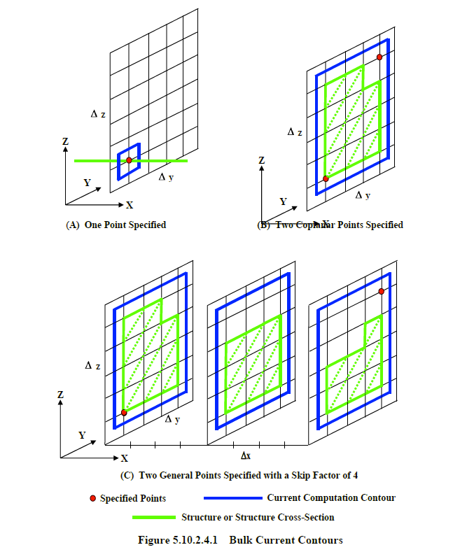
The Bulk Current Probe allows the easy computation of bulk currents through or on large structures of extended geometry such as an aircraft fuselage. With a few keywords and descriptors, many bulk current responses can be computed over a variety of structures. This includes currents on single geometric lines. The output format within the file produced by this probe is:

time, quantity1, quantity2, quantity3,…etc.

The bulk current is computed utilizing Ampere’s law. The integral path or contour is defined by points that bound a rectilinear region in which the contour exists. If only one point is specified, then the contour is as depicted by the thick blue line in Figure 5.10.2.4.11A. This is useful if current on a single PEC or conducting line is desired. If two coplanar points are specified, coplanar as in the sense of a plane perpendicular to a coordinate axis, then the contour of Figure 5.10.2.4.1B is used. If two noncoplanar points are specified, with a skip factor of 4, then the three contours of Figure 5.10.2.4.1C result. A skip factor of four implies 4 finite difference mesh increments as depicted. The contours of Figure 5.10.2.4.1C can be used to compute bulk currents at many different locations along the length of a structure.

There are two keywords associated with the Bulk Current Probe. These keywords are listed below.

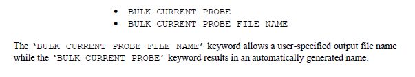
The use of the ‘Bulk Current Probe’ keyword results in an automatically generated output file name. The automatically generated name has the characters, “bpr”, concatenated onto the end of the input file base name. These characters are designed to abbreviate the Bulk Current Probe utility. The file extension of all ‘Bulk Current Probe’ output files is, “.dat”. Thus, if the input file name was, “Model1.emin”, then any ‘Bulk Current Probe’ specification will result in at least one file with the name:

“Model1bpr*.dat”

The remaining asterisk is a place-holder for an integer that numbers the files. The numbers correspond to the order of appearance of each ‘Bulk Current Probe’ specification in the EMA3D input file. Each ‘Bulk Current Probe’ specification increments this number by one. Therefore, if two ‘Bulk Current Probe’ specifications were used, then two files with the following names would be created.

“Model1bpr1.dat” “Model1bpr2.dat”

The Poynting Vector Probe allows the easy computation of the poynting vector over a rectilinear surface or from the inside to the outside of a defined rectilinear box. The different output features of include: Time domain calculations Frequency domain calculations Transfer function calculations

The pointing vector is obtained by taking the real part of the quantity, E×H*, at each mesh location over the specified surfaces and summing the result. For time domain output the quantity E×H is summed in the time domain. For frequency domain or transfer function output the above quantity is summed in the frequency domain. The units of the poynting vector are in watts/m2.

The output format for time domain information is:

time, quantity1, quantity2, quantity3,…etc.

The output format for frequency domain information is:

frequency, quantity1, quantity2, quantity3,…etc.

The pointing vector is obtained by computing E×H*at each mesh location, over the specified surfaces, and summing the result. Tangential electric fields exists on the specified surfaces. However, the associated tangential H-fields exist a half a cell on either side of the surface. These H-fields will be averaged to provide a H-field on the specified surface that is perpendicular to the associated E-field.

The frequency domain calculations are done during the computation so there is no need to store the corresponding time domain results unless desired. With the Poynting Vector Probe, one can easily specify a range or bandwidth of frequencies. In addition to frequency domain results, transfer functions (see below) can also be computed and written in the same easy format as that given above. If frequency domain information is specified, the associated time domain responses from which the frequency data is computed, should decay to a value close to zero to affect proper spectral analysis. Failure to adhere to this will compromise the spectral data.

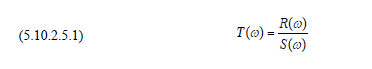
A transfer function, T(ω), is the ratio of a response, R(ω), to the driving source, S(ω), that produced the response. As indicated by the symbol, “ω”, all waveforms are in the frequency domain. This relationship is given by Equation (5.10.2.5.1.) below.

The response, R(ω), is the computed poynting vector. The driving source, S(ω), is any of those allowable within EMA3D. When using transfer functions, only one source waveform, S(ω), should be driving the model. That is, a plane wave source with no other nodal sources present, or perhaps a collection of nodal sources all utilizing the same source waveform. Multiple source waveforms will all contribute to the response, R(ω), thereby affecting the transfer function.

Inspection of Equation (5.10.2.5.1) shows a transfer function to be a normalized response. This eliminates the spectral character of the source. For example, if a plane wave source, with a particular electric field waveform, were used to drive a model, then the resultant response would be dependent upon the spectral character of the electric field waveform. Computing a transfer function would eliminate the spectral effects of the source producing a response as if CW plane waves, of 1.0 volt/meter amplitude across the band employed by the source, were driving the model.

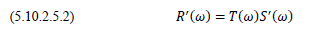
When a transfer function, T(ω), has been calculated for a particular response, R(ω), then the corresponding response, R'(ω), associated with another source, S'(ω), possessing the same geometric relationship to the geometry of the object, can be obtained using Equation (5.10.2.5.2) below.

There are two keywords associated with the Poynting Vector Probe. These keywords are listed below.

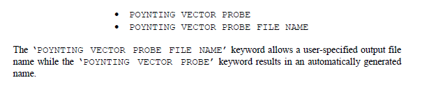
The use of the ‘POYNTING VECTOR PROBE’ keyword results in an automatically generated output file name. The automatically generated name has the characters, “pvp”, concatenated onto the end of the input file base name. These characters are designed to abbreviate the Poynting Vector Probe utility. The file extension of all POYNTING VECTOR PROBE’ output files is, “.dat”. Thus, if the input file name was, “Model1.emin”, then any POYNTING VECTOR PROBE’ specification will result in at least one file with the following name.

“Model1pvp*.dat”

The remaining asterisk is a place-holder for an integer that numbers the files. Each POYNTING VECTOR PROBE’ specification increments this number by one. Therefore, if two POYNTING VECTOR PROBE’ specifications were used, then two files with the following names would be created.

“Model1pvp1.dat” “Model1pvp2.dat”

The Regional Probe allows the easy computation of time domain field quantities within a defined volume of space. The field quantities include all three components of electric and magnetic fields. The time domain output format is:

time, quantity1, quantity2, quantity3,…etc.

The use of the ‘REGIONAL PROBE’ keyword results in an automatically generated output file name. The automatically generated name has the characters, “rgp”, concatenated onto the end of the input file base name. These characters are designed to abbreviate the Regional Probe utility. The file extension of all Regional Probe output files is, “.dat”. Thus, if the input file name was, “Model1.emin”, then any ‘REGIONAL PROBE’ specification will result in at least one file with the following name.

“Model1rgp*.dat”

The remaining asterisk is a place-holder for an integer that numbers the files. Each ‘REGIONAL PROBE’ specification increments this number by one. The numbers correspond to the order of appearance of each ‘REGIONAL PROBE’ specification in the EMA3D input file. Therefore, if two ‘REGIONAL PROBE’ were specified, then two files with the following names would be created.

“Model1rgp1.dat” “Model1rgp2.dat”

The Nonlinear Background Probe is used to write out information associated with the implementation of a nonlinear background involving the breakdown of air. The quantities written out are provided below.

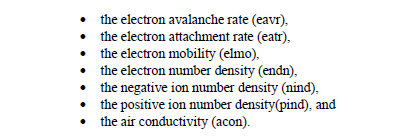
This probe can only be activated when a nonlinear background is specified. The information is written out in collimated format in the order as it appears above. The output format is therefore as shown below:

time, eavr, eatr, elmo, endn, nind, pind, acon

There are two keywords associated with the Regional Probe. These keywords are listed below.

The use of the ‘NONLINEAR BACKGROUND PROBE’ keyword results in an automatically generated output file name. The automatically generated name has the characters, “nbp”, concatenated onto the end of the input file base name. These characters are designed to abbreviate the Nonlinear Background Probe utility. The file extension of all ‘NONLINEAR BACKGROUND PROBE’ output files is, “.dat”. Thus, if the input file name was, “Model1.emin”, then any ‘NONLINEAR BACKGROUND PROBE’ specification will result in at least one file with the name:

“Model1nbp*.dat”

The remaining asterisk is a place-holder for an integer that numbers the files. Each ‘NONLINEAR BACKGROUND PROBE’ specification increments this number by one. The numbers correspond to the order of appearance of each ‘NONLINEAR BACKGROUND PROBE’ specification in the EMA3D input file. Therefore, if two ‘NONLINEAR BACKGROUND PROBE’ were specified, then two files with the following names would be created.

“Model1nbp1.dat” “Model1nbp2.dat”