Postscript

There are four probe types located in the POSTSCRIPT Probe Group. These probe types are listed below.

The Structure Probe allows the creation of POSTSCRIPT files of the meshed structure being modeled. These files can be submitted to any POSTSCRIPT printer or observed with a POSTSCRIPT viewer. One has the ability to specify what material or structures are to be included and the associated color. Many viewing parameters can be selected and controlled.

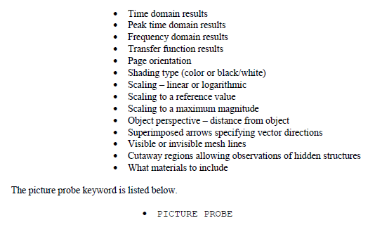
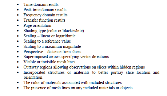
The Picture Probe feature allows the creation of detailed pictures portraying the electromagnetic behavior of the structure being modeled. The pictures consist of POSTSCRIPT files that can be submitted to any POSTSCRIPT reader or POSTSCRIPT printer. Pictures containing snapshots of time domain behavior, maximum peak values over the time of the simulation, frequency domain results, and transfer function results, on all specified materials or within specified regions, can be created. For time domain results, the pictures are created at specified times during the finite difference simulation allowing the easy monitoring of the evolving electromagnetic behavior. The choice of creating any number of pictures over any specified time or frequency range is available. Normal electric fields, normal magnetic fields, tangential electric fields, tangential magnetic fields, electric surface current densities, or magnetic surface current densities, on all structures, can be observed. A user-defined descriptive legend is provided within each picture. Many parameters can be selected and controlled such as:

When creating a pictures of frequency domain data, including transfer functions, the pictures will be created at the completion of the finite difference computation. Associated spectral analysis of time domain data is performed concurrently with the finite difference computation. For accurate spectral results, the associated time domain responses from which the frequency data is derived, should decay to a value close to zero. Failure to adhere to this will compromise the spectral data.

When implementing a Picture Probe, the coordinates of the observer are specified. This specification defines the position of the observer relative to all meshed surface elements within the model. Only those fields on the observer side of the surface are averaged. There are thus, two possible field values associated with a single surface mesh element. The value used depends upon the relative location of the observer. Field values associated with a surface element, when viewed from an exposed side, will generally possess higher values than the field values associated with the same surface element viewed from a shielded side.

There are nine electromagnetic quantities that can be plotted using the Picture Probe. A subset of these are listed below.

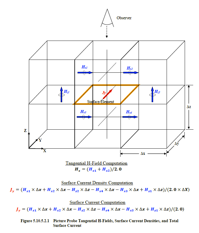
It is important to understand the difference between these three quantities because each may result in significantly different outcomes. As discussed above, tangential fields associated with a surface element are computed on the side of the element seen by the observer. The surface current density, on the other hand, is defined as the total current through that surface mesh element divided by the mesh cell spatial increment. The surface currents are just the total current through each finite difference surface mesh element. In the latter two cases, the total current is computed utilizing Amperes law. The manner of computing each of these three quantities is portrayed in Figure 5.10.5.2.1. If the surface element in the figure is one of many associated with a PEC surface (or a highly conductive surface), then the components Hz1 and Hz2 are zero (or near zero). In addition, if the opposite side of the surface from the observer is well shielded, then Hx3 and Hx4 are zero (or near zero), and the surface current density computation reduces to that of the tangential H-field.

The files created by the Picture Probe facility have the characters, “ppr”, concatenated onto the end of the input file base name. The Picture Probe output file is a POSTSCRIPT file. The file extension of all EMA3D® POSTSCRIPT files is “.ps”. Thus, if the input file name was, “Model1.emin”, then any Picture Probe specification will result in a file with the name:

“Model1ppr#-****.ps”

The number character, '#' and asterisks '*' stand for other characters yet to be explained.

For the Picture Probe utility, time domain results, peak magnitude time domain results, frequency domain results, and transfer function results, can be specified. If time domain information is specified, then the characters, “timepict”, are concatenated onto the end of the file base name, producing the result:

“Model1ppr#-timepict*.ps”

If peak magnitude time domain information is specified, then the characters, “peakpict”, are concatenated onto the end of the file base name, producing the result:

“Model1ppr#-peakpict*.ps”

If frequency domain information is specified, then the characters, “freqpict”, are concatenated onto the end of the file base name, producing the result:

“Model1ppr#-freqpict*.ps”

If transfer function information is specified, then the characters, “tranpict”, are concatenated onto the end of the file base name, producing the result:

“Model1ppr#-tranpict*.ps”

The number character, '#', is a place-holder for an integer that numbers the Picture Probe specifications. The asterisk, '*', is a place-holder for an integer that numbers the output files for each particular Picture Probe specification. Thus if a two time domain Picture Probe were specified within the EMA3D input file named, 'Model1.emin', with the first Picture Probe producing 3 POSTSCRIPT files and the second one producing 4 POSTSCRIPT files, then the following files names would be produced.

“Model1ppr1-timepict000001.ps” “Model1ppr1-timepict000002.ps” “Model1ppr1-timepict000003.ps” “Model1ppr2-timepict000001.ps” “Model1ppr2-timepict000002.ps” “Model1ppr2-timepict000003.ps” “Model1ppr2-timepict000004.ps”

The Slice Probe is a powerful algorithm that allows the creation of pictures depicting the electromagnetic behavior on spatial slices through the finite difference problem space. Like the Picture Probe, these pictures consist of POSTSCRIPT files, that can be submitted to any POSTSCRIPT printer. Snapshots of time domain behavior, maximum peak values over a specified time range, frequency domain results, and transfer function results can be created. For time domain results, the pictures are created at user-specified times during the finite difference computation allowing easy monitoring of the evolving electromagnetic behavior. The choice of creating any number of pictures over any specified time or frequency range is available. On any slice, normal electric fields, normal magnetic fields, tangential electric fields, tangential magnetic fields, total electric fields, or total magnetic fields can all be monitored. If a nonlinear background is specified, then the spatial charge can be observed. Geometric structures or materials can be included along with the slices to provide descriptive depictions of slice location and orientation. A user-defined descriptive legend is provided within each picture. Many parameters can be selected and controlled such as:

When creating a picture of frequency domain data, including transfer functions, the picture will be created at the completion of the finite difference computation. Associated spectral analysis of time domain data is performed concurrently with the finite difference computation. For accurate spectral results, the associated time domain responses from which the frequency data is computed should decay to a value close to zero. Failure to adhere to this will compromise the spectral data.

The files created by the Slice Probe facility have the characters, “spr”, concatenated onto the end of the input file base name. The Slice Probe output file is a POSTSCRIPT file. The file extension of all EMA3D POSTSCRIPT files is “.ps”. Thus, if the input file name was, “Model1.emin”, then any Slice Probe specification will result in a file with the name:

“Model1spr#-****.ps”

The number character, '#' and asterisks '*' stand for other characters yet to be explained. For the Slice Probe utility, time domain results, peak magnitude time domain results, frequency domain results, or transfer function results, can be specified. If time domain information is specified, then the characters, “timepict”, are concatenated onto the end of the file base name, producing the result

“Model1spr#-timepict*.ps”

If peak magnitude time domain information is specified, then the characters, “peakpict”, are concatenated onto the end of the file base name, producing the result:

Model1spr#-peakpict*.ps”

If frequency domain information is specified, then the characters, “freqpict”, are concatenated onto the end of the file base name, producing the result:

“Model1spr#-freqpict*.ps”

If transfer function information is specified, then the characters, “tranpict”, are concatenated onto the end of the file base name, producing the result:

“Model1spr#-tranpict*.ps”

The number character, '#', is a place-holder for an integer that numbers the Slice Probe specifications. The asterisk, '*', is a place-holder for an integer that numbers the output files for each particular Slice Probe specification. Thus if a two time domain Slice Probes were specified within the EMA3D input file named, "Model1.emin", with the first Slice Probe producing 3 POSTSCRIPT files and the second one producing 4 POSTSCRIPT files, then the following files names would be produced.

“Model1spr1-timepict000001.ps” “Model1spr1-timepict000002.ps” “Model1spr1-timepict000003.ps” “Model1spr2-timepict000001.ps” “Model1spr2-timepict000002.ps” “Model1spr2-timepict000003.ps” “Model1spr2-timepict000004.ps”

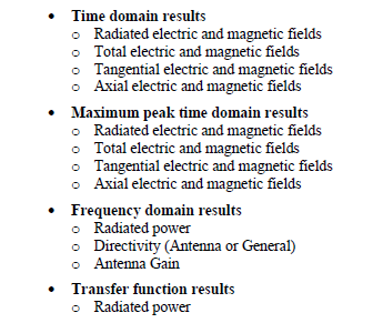
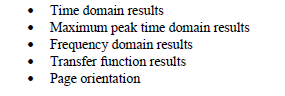
The Radiation Pattern Probe is a powerful algorithm that allows the creation of pictures depicting the nature of electromagnetic radiation patterns at great distances beyond the confines of the finite difference problem space. Like the Picture Probe and the Slice Probe, these pictures consist of POSTSCRIPT files that can be submitted to any POSTSCRIPT printer. Snapshots of time domain behavior, maximum peak time domain values over a specified time range, frequency domain results, and transfer function results can be created. The frequency domain results can consists of radiated power, radiated power transfer functions, directivity, and antenna gain patterns. These quantities are computed on a sphere with a user defined radius and various angular specifications. A complete list of result types is provided below.

For time domain results, the pictures are created at user-specified times during the finite difference computation allowing easy monitoring of the evolving electromagnetic behavior. The choice of creating any number of pictures over any specified time or frequency range is available. Geometric structures or materials can be included along with the patterns to provide descriptive depictions of pattern orientation.

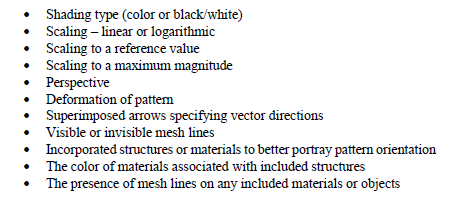
Three-dimensional patterns, as well as two-dimensional patterns, can be created at user defined angular resolutions. The pattern can be calculated at great distances and then drawn at close proximity, around the structures being modeled, to provide the proper geometric relationship for enhanced visual effects. A user-defined descriptive legend is provided within each picture. Many parameters can be selected and controlled such as:

To compute quantities associate with the Radiation Pattern Probe requires the presence of a rectilinear equivalent integration surface. To calculate the various Radiation Pattern Probe quantities requires the computation of electric and magnetic surface current densities on the specified equivalent surface. These current densities are synthesized, with proper retardation times, to provide the electric and magnetic fields on the specified Radiation Pattern Probe spherical surface at the designated angular locations.

The Radiation Pattern Probe equivalent surface must be contained within the finite difference problem space and should surround all structures being modeled. The background material must be a vacuum (or air). It is best to specify a surface that is at least five cells from any structures within the problem space. However, the larger the number of cells constituting the rectilinear volume, the more computationally intensive the simulation, and the greater the amount of CPU time required.

Time domain pictures are created at user specified times. These times are associated with the simulation computations and do not include the propagation time to the distant locations where the pattern quantities are being computed. The first nonzero quantities computed occur when the first nonzero fields reach the Radiation Pattern Probe equivalent surface.

When creating a picture of frequency domain data, including transfer functions, the picture will be created at the completion of the finite difference computation. Associated spectral analysis of time domain data is performed concurrently with the finite difference computation. For accurate spectral results, the associated time domain responses from which the frequency data is computed should decay to a value very close to zero. Five orders of magnitude down from the peak is usually sufficient. Failure to adhere to this will compromise the spectral data.

For many finite difference applications, ten mesh cells may be used to resolve the highest frequency (smallest wavelength) of interest. However, for antenna gain and directivity computations a greater number of cells may need to be employed. A recommended number is around thirty. Therefore, if a 100 MHz antenna is being modeled, then a mesh size no greater than of 10 cm (4 inches) should be used.

The directivity computation requires the specification of polar and azimuthal angular increments over a three-dimensional sphere to compute the total radiated power. The angular increments must cover the entire sphere. The smaller the angular increments, and the larger the Radiation Pattern Probe rectilinear surface, the more computationally intensive the problem becomes. For large problems, it may prove useful to start with angular increments of 30 degrees to test the speed of computation and then reduce to smaller values.

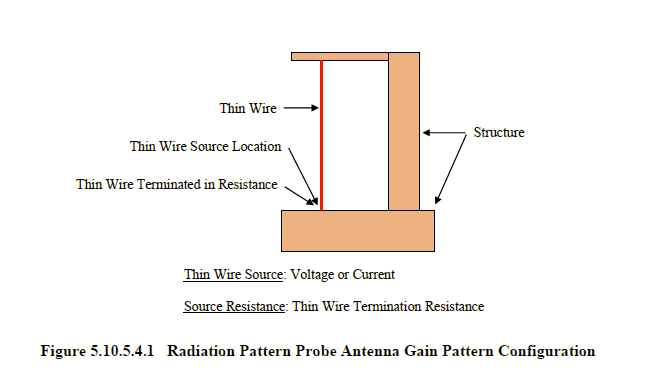
To compute antenna gain patterns requires the presence of a thin wire and a thin wire source. The thin wire source can be specified as a voltage source or a current source. A source resistance must also be specified. A descriptive configuration is illustrated in Figure 5.10.5.4.1. There can only be one thin wire source applied at one location on a thin wire. No other sources are allowed. If other sources are present, then an error will result and EMA3D will terminate.

Three parameters are required for antenna gain pattern computations. These parameters are described in Figure 5.10.5.4.1 and are listed below.

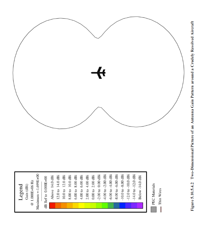
The Radiation Pattern Probe can produce two-dimensional and three-dimensional patterns. A two-dimensional antenna gain pattern around a crudely resolved aircraft is shown in Figure 5.10.5.4.2. This pattern is associated with an antenna along the front edge of the vertical stabilizer. The two-dimensional pattern exists in the xy-plane (normal z-direction) and is viewed along the z-coordinate axis.

Two parameters are required to define a two-dimensional pattern. These parameters are listed below.

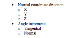
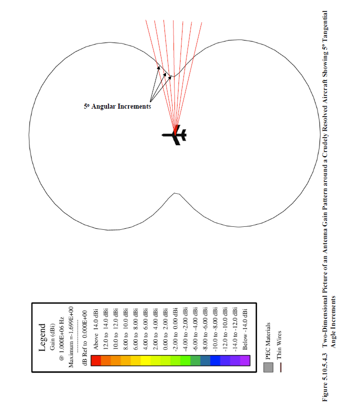
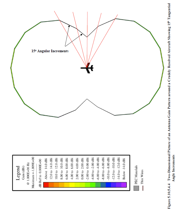
The normal coordinate direction is self-explanatory. There are only three choices, "X", "Y", "Z". There are also two angle increments that need to be defined. The tangential increment concerns the resolution of the two dimensional pattern illustration. The tangential increment for the two-dimensional pattern in Figure 13.2.4.2 was 5o. The pattern of Figure 5.10.5.4.2 is duplicated in Figure 5.10.5.4.3 with the 5o increment superimposed on top. The pattern with a 15o increment is shown in Figure 5.10.5.4.4.

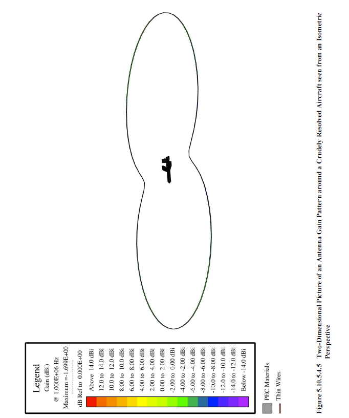
The pictures of Figure 5.10.5.4.2 through Figure 5.10.5.4.4 are two-dimensional depictions normal to the z-axis and viewed along that same axis. Although the depictions are normal to the z-axis, the viewing location does not have to be. The pattern of Figure 5.10.5.4.2 is viewed from a different perspective in Figure 5.10.5.4.5.

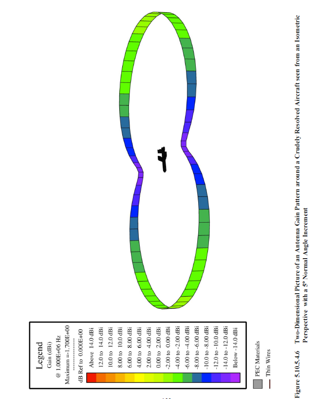
The normal angle increment concerns the angular thickness of the pattern in the normal coordinate direction of the two-dimensional depiction. The gain pattern of Figure 5.10.5.4.5 has a small normal angle increment. The same illustration with a 5o normal angle increment is shown in Figure 5.10.5.4.6. The reason for the legend in Figure 5.10.5.4.5 is now apparent where it may have been somewhat obscured in the other figures.

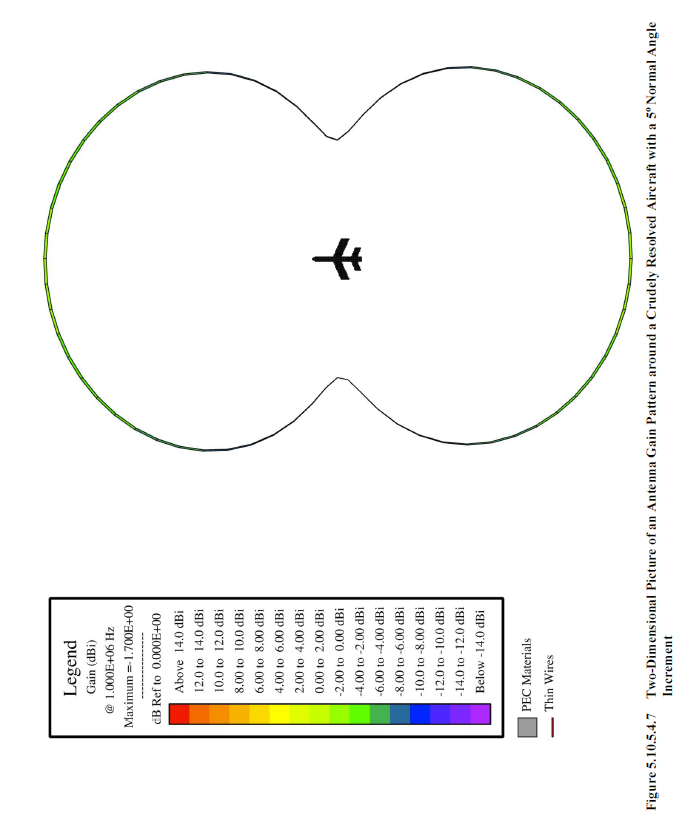
When viewing along a coordinate direction it is usually best to keep the normal angle at a small value such as 0.5o or less. This will create a crisp two-dimensional pattern. The gain pattern of Figure 5.10.5.4.6, possessing a 5o normal angle increment, when viewed along the z-axis results in the picture seen in Figure 5.10.5.4.7. Compare this with Figure 5.10.5.4.2.

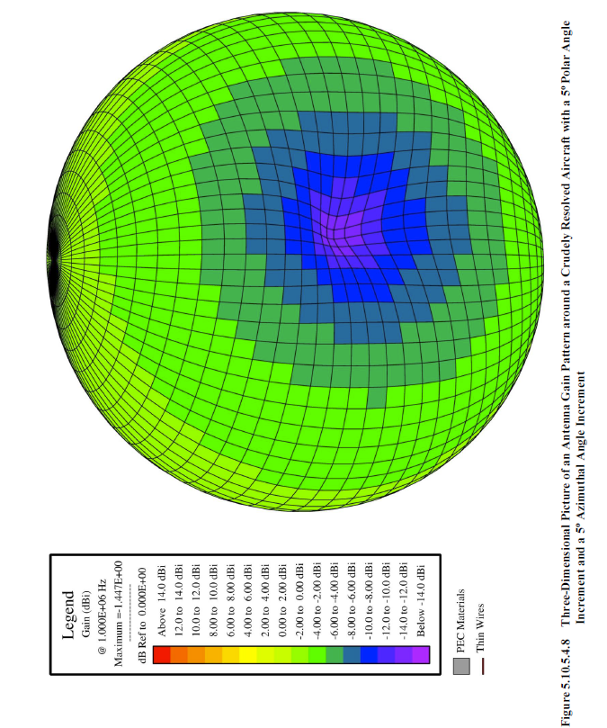
For three dimensional patterns a polar angle increment and an azimuthal angle increment must be specified. The polar angle is measured from the positive z-coordinate axis of the model coordinate system and the azimuthal angle is measured from the positive x-coordinate. A full three-dimensional gain pattern viewed from the same perspective as that of Figure 5.10.5.4.6, using a 5o polar angle increment and a 5o azimuthal angle increment, is shown in Figure 5.10.5.4.8.

There are two different calculation types. These type are labeled, 'SLOW' and 'FAST''. The 'FAST' option is significantly quicker than the 'SLOW' option, but requires substantially more memory. This memory is proportional to the angle increments defined and the size of the equivalent surface. For two-dimensional depictions, the memory is usually not a problem. However, for three-dimensional illustrations the memory can be prohibitive.

When implementing the 'FAST' option on parallel processing, all processors will be assigned the same memory. If multiple processors use the same RAM memory, then the 'FAST' option may prove prohibitive.

The calculation distance is the radial distance at which the Radiation Pattern Probe quantities are computed. However, the pattern does not have to be drawn at this particular distance. The pattern can be specified to be drawn at any radial distance. This is the function of the "drawing distance". The desire may be to compute a quantity in the far field regime but illustrate the pattern at a distance where the radiating structure is easily discernible, thereby producing an image portraying the physical relationship between the structure and the pattern.

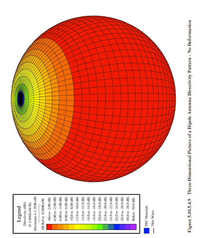
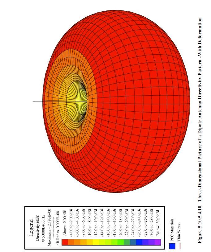
The deformation factor allows the radiation pattern to be deformed. The directivity pattern of a radiating dipole is seen in Figure 5.10.5.4.9. This illustration is not deformed and only the colors on the sphere reveal the pattern. Inspection of Figure 5.10.5.4.9 reveals values at the poles to be more than 20dB down from those at the equator. The deformation factor specifies the value required to result in full deformation, that is, full collapse to the center of the sphere. Therefore, a deformation factor of 20 (in dB) applied to the pattern of Figure 5.10.5.4.9 would fully deform or collapse the sphere at the poles resulting in the deformed illustration of Figure 5.10.5.4.10.

The observer coordinate system can only be specified as "Spherical". The radial distance associated with a spherical specification must exceed the drawing distance discussed earlier.

The files created by the Radiation Pattern Probe facility have the characters, “rpp”, concatenated onto the end of the input file base name. There are two type of files put out by the Radiation Pattern Probe. One type is a POSTSCRIPT file, the other type is a data file. The data file is created if so specified. The file extension of all EMA3D POSTSCRIPT files is “.ps”. Thus, if the input file name was, “Model1.emin”, then any Radiation Pattern Probe specification will result in a file with the name:

The number character, '#' and asterisks '*' stand for other characters yet to be explained.

Part of the asterisk character field depends on the Radiation Pattern Probe quantity to be plotted. There are twenty different quantities. These quantities are listed below along with the associated descriptive character fields used in the asterisk field.

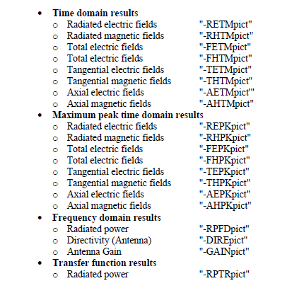
If time domain radiated field information is specified, then the characters, “-RETMpict”, are concatenated onto the end of the file base name, producing the result:

“Model1rpp#-RETMpict*.ps”

The number character, '#', is a place-holder for an integer that numbers the Radiation Pattern Probe specifications. The asterisk, '*', is a place-holder for an integer that numbers the output files for each particular Radiation Pattern Probe specification. Therefore, if two time domain radiated field probes were specified within the EMA3D input file named, 'Model2.emin', with the first Radiation Pattern Probe producing 3 POSTSCRIPT files and the second one producing 4 POSTSCRIPT files, then the following files names would be produced.

“Model2rpp1-RETMpict000001.ps” “Model2rpp1-RETMpict000002.ps” “Model2rpp1-RETMpict000003.ps” “Model2rpp2-RETMpict000001.ps” “Model2rpp2-RETMpict000002.ps” “Model2rpp2-RETMpict000003.ps” “Model2rpp2-RETMpict000004.ps”