Specialty

There are four probe types associated with the Specialty Probe Group. These probe types are listed below.

Each of these probes is discussed in separate subsections below.

The Box In Probe is used to create the file containing the electric and magnetic fields to be used when specifying a Box In Source (see Section 5.6.1.2).

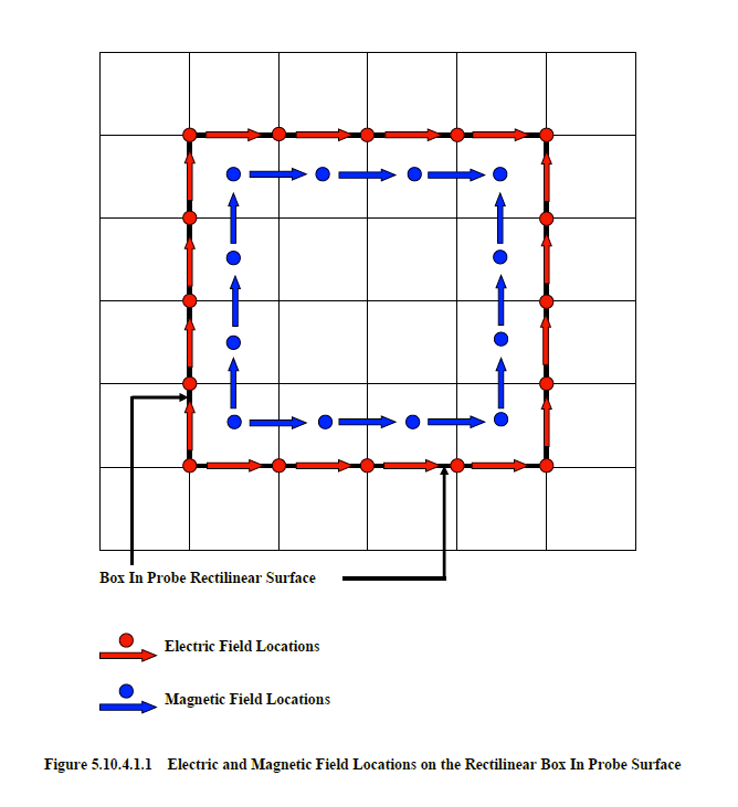
Implementation of the Box In Probe results in the generation of a file containing the electric and magnetic fields on a specified rectilinear surface. This surface, along with the electric and magnetic fields, is shown in the two-dimensional representation of Figure 5.10.4.1.1. The Box In Probe is actually the first step of a two-step process. The second step is associated with the Box In Source discussed in Section 5.6.1.2. Within Section 5.6.1.2, is a description of the overall technique and the introduction of terminology. There can be as many Box In Probe specifications as desired.

When specifying a Box In Probe, it is best to avoid material penetrations as much as possible. This includes any penetrations by more than one background. The interpolation scheme used when applying the Box In Source is less accurate in regions closest to material penetrations. Therefore, the rectilinear surface should be defined to avoid penetrations as much as possible. If any portion of the rectilinear surface is exterior to the finite difference problem space bounds, an error message will result and the program will terminate.

For any Box In Probe output, the characters, “bip”, are concatenated onto the end of the input file base name. These particular characters are designed to abbreviate the Box In Probe utility. The file extension of all Box In Probe output files is, “.dat”. Thus, if the input file name was, “Model1.emin”, then any Box In Probe specification will result in at least one file with the name:

“Model1bip*.dat”

The remaining asterisk is a place-holder for an integer that numbers the files. Each Box In Probe specification increments this number by one. The numbers correspond to the order of appearance of each Box In Probe specification in the EMA3D® input file. Therefore, if two Box In Probes were specified, then two files with the following names would be created.

“Model1bip1.dat” “Model1bip2.dat”

The Box Out Probe is used to create the file containing the electric and magnetic fields to be used when specifying a Box Out Source (see Section 5.6.1.3).

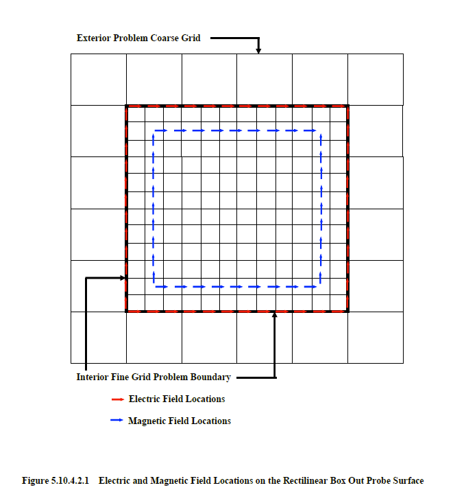
Implementation of the Box Out Probe results in the generation of a file containing the electric and magnetic fields on a specified rectilinear surface. This surface, along with the electric and magnetic fields, is shown in the two-dimensional representation of Figure 5.10.4.2.1. The Box Out Probe is actually the first step of a two-step process. The second step is associated with the Box Out Source discussed in Section 5.6.1.3. Within Section 5.6.1.3, is a description of the overall technique and the introduction of terminology. There can be as many Box Out Probe specifications as desired.

Before implementing a Box Out Probe it is necessary to know the expansion factor required by the Box Out Source. The output fields of the Box Out Probe are averaged according to the expansion factor (see Section 5.6.1.3).

When specifying a Box Out Probe, it is best to avoid material penetrations as much as possible. This includes any penetrations by more than one background. The interpolation scheme used when applying the Box Out Source is less accurate in regions closest to material penetrations. Therefore, the rectilinear surface should be defined to avoid penetrations as much as possible. If any portion of the rectilinear surface is exterior to the finite difference problem space bounds, an error message will result in EMA3D and the program will terminate.

For any Box Out Probe output, the characters, “bop”, are concatenated onto the end of the input file base name. These characters are designed to abbreviate the Box Out Probe utility. The file extension of all Box Out Probe output files is, “.dat”. Thus, if the input file name was, “Model1.emin”, then any Box Out Probe specification will result in at least one file with the name:

“Model1bop*.dat”

The remaining asterisk is a place-holder for an integer that numbers the files. Each Box Out Probe specification increments this number by one. The numbers correspond to the order of appearance of each Box Out Probe specification in the EMA3D input file. Therefore, if two Box Out Probes were specified, then two files with the following names would be created.

“Model1bop1.dat” “Model1bop2.dat”

The Far Field Probe can be used to obtain electric and magnetic field data at far field points. These point locations may be within the finite difference problem space or at great distances from the confines of the problem space. The far field algorithm computes the total field, including the near field, the inductive field, and the far field. For true far field analysis, the points should be located far outside of, or beyond, the problem space boundaries.

The locations of far fields are specified using spherical coordinates. With a set radial distance, the far field locations over a sphere can be defined using a start, stop, and step values for the polar angle and the azimuthal angle.

The far field algorithm operates by computing electric and magnetic surface current densities on a specified far field integration surface. These current densities are synthesized, with the proper retardation times, to provide the far field electric fields at close or at distance points from the far field surface. The Far Field Probe thus requires the specification of the far field integration surface.

There are two algorithms used to compute far field electric fields. One algorithm performs the computations significantly more quickly but uses substantially more memory. In some cases, the required memory may exceed that of the computing machine. In this case, the slower algorithm should be used.

The Far Field probe cannot be applied to two-dimensional problems, used in conjunction with a gamma source, used when a plane wave/lossy ground configuration is specified, when periodic boundary conditions are designated, or when symmetric boundaries on opposite boundaries are present. A PEC ground is permissible, but only on one side of the finite difference problem space. This includes grounds specified by PEC boundary conditions. The far field integration surface cannot be employed with an electrically or magnetically conductive background medium. The far field integration surface must also be contained within the finite difference problem space. Violating any of these conditions, results in error messages in EMA3D and program termination.

If a PEC, PMC, or symmetric boundary is specified, then the far field integration surface must contact this boundary. If this is violated, then the surface will be automatically modified to provide contact. For accurate results, the far field integration surface should be placed no closer than five cells from the finite difference problem space bounds when quasi-static or absorbing boundary conditions are employed. An exception is when PML boundaries are employed. In this case, the surface can be placed as close as one cell away.

The far field integration surface, in most cases, should contain all electromagnetic sources within the problem. The surface should therefore contain the plane wave source equivalent surface, the Box In Source equivalent surface, or the Box Out Source equivalent surface, if such are present.

When defining a far field integration surface, it is best to avoid material penetrations of the surface as much as possible. This includes any penetrations by more than one background. If any materials do penetrate, a warning message will be issued in EMA3D.

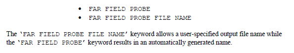
The use of the ‘FAR FIELD PROBE’ keyword results in an automatically generated output file name. The automatically generated name has the characters, “ffp”, concatenated onto the end of the input file base name. These characters are designed to abbreviate the Far Field Probe utility. The file extension of all ‘FAR FIELD PROBE’ output files is, “.dat”. Thus, if the input file name was, “Model1.emin”, then any ‘FAR FIELD PROBE’ specification will result in at least one file with the name:

“Model1ffp*.dat”

The remaining asterisk is a place-holder for an integer that numbers the files. Each ‘FAR FIELD PROBE’ specification increments this number by one. The numbers correspond to the order of appearance of each ‘FAR FIELD PROBE’ specification in the EMA3D input file. Therefore, if two ‘FAR FIELD PROBE’ were specified, then two files with the following names would be created.

“Model1ffp1.dat” “Model1ffp2.dat”

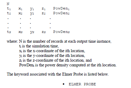
The Elmer Heat Probe is used to create a file to be read by the Elmer Heat Program (see appropriate documentation). This file contains coordinate information and associated power density values to be used by the Elmer Heat program to analyze heat accumulation and dissipation. The format of the EMA3D output file containing the required information for the Elmer Program is provided below.

For any Elmer Heat Probe output, the characters, “elmheat”, are concatenated onto the end of the input file base name. These characters are designed to abbreviate the Elmer Heat Probe utility. The file extension of all Elmer Heat Probe output files is, “.dat”. Thus, if the EMA3D input file name was, “Model1.emin”, then any Elmer Heat Probe specification will result in at least one file with the name:

“Model1elmheat*.dat”

The remaining asterisk is a place-holder for an integer that numbers the files. The numbers correspond to the order of appearance of each Elmer Heat Probe specification in the EMA3D input file. Every Elmer Heat Probe specification increments this number by one. Therefore, if two Elmer Heat Probes were specified, then two files with the following names would be created.

“Model1elmheat1.dat” “Model1elmheat2.dat”