Traditional

The Traditional Probe is so named because it was the only probe type available in earlier versions of EMA3D®. The primary function of the Traditional Probe is to produce results for post-processing or visualization purposes within a previous GUI, such as response animations. However, the functionality of the Traditional Probe has been superseded by other probes (see X vs T). Although the Traditional probe is still present in EMA3D version 7, it may be eliminated in future versions. With the Traditional Probe, EMA3D output can be obtained for the following entities.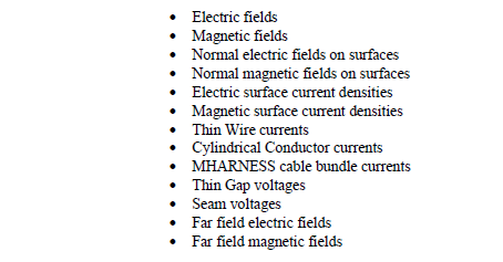

Each of the above Traditional Probe entities are discussed in separate subsections below.

The Traditional Electric Field Probe can be used to obtain electric field data. The electric field output provided is the average at the center of a finite difference mesh cell. The electric field components, superimposed on a finite difference mesh cell, is shown in Figure 5.10.1.1.1. A representative set of the magnetic field components is also included for clarity. To provide one electric field component at the center of a finite difference mesh cell requires averaging of the four associated electric field components at the edges of the cell faces. Since Traditional Electric Field Probes record three field components, three sets of four fields require averaging.

The averaging technique described above is satisfactory in most cases. However, the analyst should be aware that such is occurring. If a field component at the tip of a metal isotropic line is desired, the Traditional Electric Field Probe result will consist of an average of four component fields, as illustrated in Figure 5.10.1.1.1. This will result in a recorded field less than the actual field at the metal line tip. If only one component is of interest, then the New Probe facility should be used.

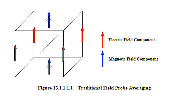
The Traditional Magnetic Field Probe can be used to obtain magnetic field data. The magnetic field output provided is the average at the center of a finite difference mesh cell. The magnetic field components, superimposed on a finite difference mesh cell, was shown in Figure 5.10.1.1.1. To provide one magnetic field component requires the averaging of the two associated magnetic field components normal to the appropriate cell faces. Since a Traditional Magnetic Field Probe supplies three field components, three sets of two fields require averaging.

The averaging technique described above is satisfactory in most cases. However, the analyst should be aware that such is occurring. If a field component at the tip of a PMC isotropic line is desired, the Traditional Magnetic Field Probe result will consist of an average of two component fields, as illustrated in the figure. This will result in a recorded field less than the actual field at the line tip. If one component field is of interest, then the New Probe facility should be used.

The Traditional Normal Electric Field Probe can be used to obtain normal electric field data on material surfaces. The normal electric field output provided is the average electric field at the center of a finite difference mesh cell face. The configuration is shown in in Figure 5.10.1.1.3. A representative set of the magnetic field components is also included for clarity. Since there is no generally preferred normal direction associated with a particular mesh cell face, fields on both sides are included in the averaging algorithm. Therefore, to provide a normal electric field at a mesh cell face requires the averaging of eight normal electric fields – four on each side, as depicted.

The averaging technique described above is satisfactory in many cases. However, the analyst should be aware that such is occurring. If a field component on one side of a surface is desired, the Traditional Normal Electric Field Probe result will consist of an average of four component fields on each side, as illustrated in the figure. If one side were shielded, perhaps on the interior of an enclosure, then the recorded normal field values would be approximately one half of the actual value. If a normal component on one side is desired, then the New Probe facility can be used.

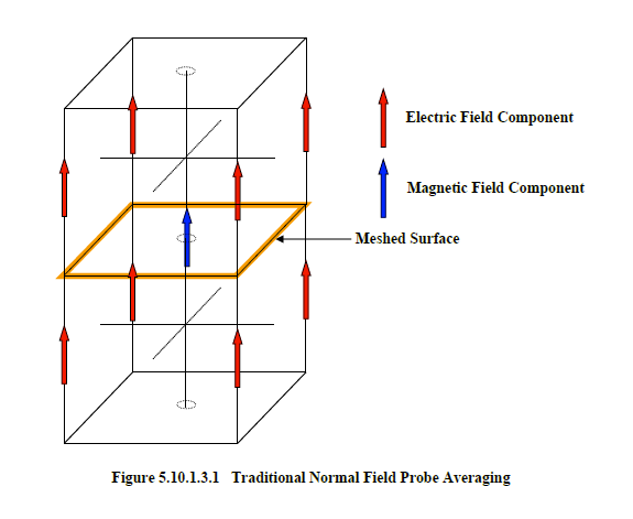
The Traditional Normal Magnetic Field Probe can be used to obtain normal magnetic field data on material surfaces. The normal magnetic field output provided is the average magnetic field at the center of a finite difference mesh cell face. The configuration was shown in in Figure 5.10.1.1.3. Examination of this figure reveals the magnetic field to be properly placed. However, a normal magnetic field, in general, contains limited information when applied to electric materials. When applied to magnetic materials, a problem arises due to material swelling (see Section 4.4). A review of that section reveals the normal magnetic field of Figure 5.10.1.1.3 to be embedded within the magnetic surface material after the swelling. This may lead to inaccurate results in many cases. To alleviate this problem one should select the magnetic field one cell above or below the material surface.

The Traditional Electric Surface Current Density Probe can be used to obtain electric surface current density data on material surfaces. Electric surface current densities are derived from magnetic field components that are parallel to the surface and in close proximity. A representative set of these tangential magnetic field components are shown superimposed between two finite difference mesh cells in Figure 5.10.1.5.1. Two representative tangential electric field components are also included for clarity. There is no generally preferred normal direction associated with a mesh cell face, so fields on both sides are included in the synthesizing algorithm. To provide an electric surface current density component at a surface mesh location requires the difference of the average tangential magnetic fields on either side. Since a Traditional Electric Surface Current Density Probe supplies two current density components, then two sets of four fields must be synthesized.

The averaging/difference technique described above is satisfactory in many cases. However, the analyst should be aware that such is occurring. If an electric surface current density on a PEC material surface is desired, the Traditional Electric Surface Current Density Probe will compute only one set of surface current density components associated with that particular surface cell face. Therefore, when the PEC surface is viewed from either side, the same surface current density values are observed. If one side were shielded, perhaps on the interior of an enclosure, then the computed surface current density values would apply to both the shielded and the unshielded side.

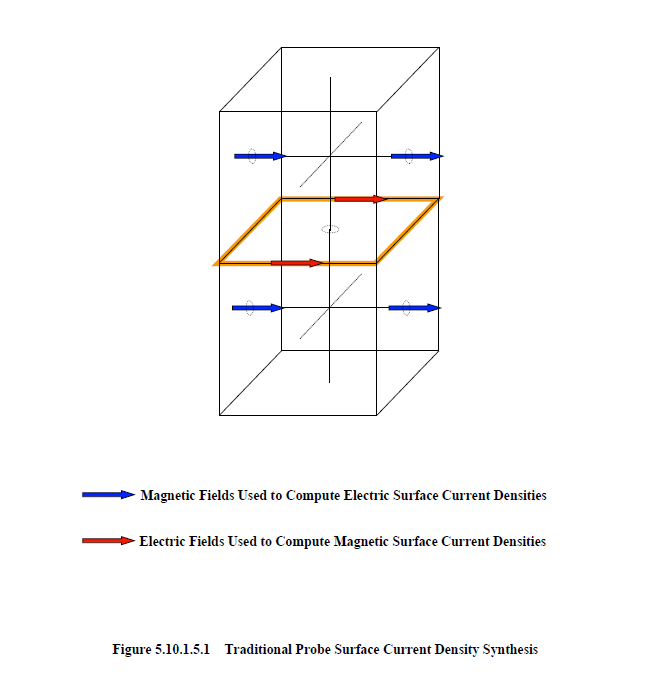
The Traditional Magnetic Surface Current Density Probe can be used to obtain magnetic surface current density data on material surfaces. The magnetic surface current density output provided is obtained using the average electric field at the center of a finite difference mesh cell face. The configuration was shown in in Figure 5.10.1.5.1. Examination of this figure reveals the tangential electric fields to be properly placed. However, a magnetic surface current density, in general, contains limited information when applied to electric materials. When applied to magnetic materials, a problem arises due to material swelling (see Section 4.4). A review of that section reveals the tangential electric fields of Figure 5.10.1.5.1 to be embedded within the magnetic surface material after the swelling. This may lead to inaccurate results in many cases. To alleviate this problem one should select the cell face one cell above or below the surface mesh cell

The Traditional Probe Thin Wire Current Probe can be used to obtain thin wire current data at any location on thin wires. The location of the wire current is specified by the identifying number attached to the thin wire meshed increment in the EMA3D input file.

The Traditional Cylindrical Conductor Current Probe can be used to obtain cylindrical conductor current data at any location on cylindrical conductors. The location of the conductor current is specified by the identifying number attached to the cylindrical conductor meshed increment in the EMA3D input file.

The Traditional MHARNESS Cable Bundle Current Probe can be used to obtain MHARNESS cable bundle currents on any exposed segment in the MHARNESS cable bundle system (see the MHARNESS User Manual). The location of the cable bundle current is specified by the identifying number attached to the MHARNESS segment meshed increment in the EMA3D input file.

The Traditional Thin Gap Voltage Probe is used to obtain voltage data at any location across thin gaps. The location is specified by using the identifying number attached to the thin gap meshed increment in the EMA3D input file.

The Traditional Probe seam voltage is used to obtain voltage data at any location across old seams. The location is specified by using the identifying number attached to the seam meshed increment in the EMA3D input file.

The Traditional Probe far field electric field utility is used to obtain electric field data at far field points. These point locations may be within the finite difference problem space or at great distances from the confines of the problem space. The locations of far field electric fields are specified by identifying the Cartesian coordinates of the far field locations. The locations can be anywhere inside or outside of the problem space. The far field algorithm computes the total field, including the near field, the inductive field, and the far field. For true far field analysis, the points should be located far outside of, or beyond, the problem space boundaries.

The Tradition Probe far field electric field algorithm operates by computing electric and magnetic surface current densities on a specified far field integration surface. These current densities are synthesized, with the proper retardation times, to provide the far field electric fields at close or at distance points from the far field surface.

There are two algorithms used to compute far field electric fields. One algorithm performs the computations significantly more quickly but uses substantially more memory. In some cases, the required memory may exceed that of available resources. In this case, the slower algorithm should be used.

The Traditional Probe far field utility cannot be applied to two-dimensional problems, used in conjunction with a gamma source, used when a plane wave/lossy ground configuration is specified, when periodic boundary conditions are designated, or when symmetric boundaries on opposite boundaries are present. A PEC ground is permissible, but only on one side of the finite difference problem space. This includes grounds specified by PEC boundary conditions. The far field integration surface cannot be employed with an electrically conductive or magnetically conductive background medium. The far field integration surface must also be contained within the finite difference problem space. Violating any of these conditions, results in error messages and program termination.

If a PEC, PMC, or symmetric boundary is specified, then the far field integration surface must contact this boundary. If this is violated, then the surface will be automatically modified to provide contact. For accurate results, the far field integration surface should be placed no closer than five cells from the finite difference problem space bounds when quasi-static or absorbing boundary conditions are employed. An exception is when PML boundaries are employed. For this case, the surface can be placed as close as one cell away.

The far field equivalent surface, in most cases, should contain all electromagnetic sources within the problem. The surface should therefore contain the plane wave equivalent surface, the Box In Source equivalent surface, or the Box Out Source equivalent surface, if such are present.

When defining a far field integration surface, it is best to avoid material penetrations of the surface as much as possible. This includes any penetrations by more than one background. If any materials do penetrate, a warning message will be issued in EMA3D.

There is also a separate Far Field Probe (see Section 5.10.4.3) with enhanced functionality. This probe is preferred and should be used, if appropriate, in place of the Traditional Probe far field electric field utility

The Traditional Probe far field magnetic field utility is used to obtain magnetic field data at far field points. These point locations may be within the finite difference problem space or at great distances from the confines of the problem space. The locations of far field magnetic fields are specified by identifying the Cartesian coordinates of the far field locations. The locations can be anywhere inside or outside of the problem space. The far field algorithm computes the total field, including the near field, the inductive field, and the far field. For true far field analysis, the points should be located far outside of, or beyond, the problem space boundaries.

The Tradition Probe far field electric field algorithm operates by computing electric and magnetic surface current densities on a specified far field integration surface. These current densities are synthesized, with the proper retardation times, to provide the far field electric fields at close or at distance points from the far field surface.

There are two algorithms used to compute far field electric fields. One algorithm performs the computations significantly more quickly but uses substantially more memory. In some cases, the required memory may exceed that of available resources. In this case, the slower algorithm should be used.

The Traditional Probe far field utility cannot be applied to two-dimensional problems, used in conjunction with a gamma source, used when a plane wave/lossy ground configuration is specified, when periodic boundary conditions are designated, or when symmetric boundaries on opposite boundaries are present. A PEC ground is permissible, but only on one side of the finite difference problem space. This includes grounds specified by PEC boundary conditions. The far field integration surface cannot be employed with an electrically conductive or magnetically conductive background medium. The far field integration surface must also be contained within the finite difference problem space. Violating any of these conditions, results in error messages and program termination.

If a PEC, PMC, or symmetric boundary is specified, then the far field integration surface must contact this boundary. If this is violated, then the surface will be automatically modified to provide contact. For accurate results, the far field integration surface should be placed no closer than five cells from the finite difference problem space bounds when quasi-static or absorbing boundary conditions are employed. An exception is when PML boundaries are employed. For this case, the surface can be placed as close as one cell away.

The far field equivalent surface, in most cases, should contain all electromagnetic sources within the problem. The surface should therefore contain the plane wave equivalent surface, the Box In Source equivalent surface, or the Box Out Source equivalent surface, if such are present.

When defining a far field integration surface, it is best to avoid material penetrations of the surface as much as possible. This includes any penetrations by more than one background. If any materials do penetrate, a warning message will be issued in EMA3D.

There is also a separate Far Field Probe (see Section 5.10.4.3) with enhanced functionality. This probe is preferred and should be used, if appropriate, in place of the Traditional Probe far field magnetic field utility.