Frequency Dependent |
Frequency dependent materials in EMA3D are always electromagnetically isotropic and linear. Both electric and magnetic frequency dependent materials are allowed. Frequency dependent materials are characterized by the static conductivity (σ0), the infinite frequency permittivity (ε∞), the infinite frequency permeability (μ∞), and the static magnetic conductivity (σm0), along with the sum of any number of first and second order rational functions. Utilizing complex expressions for the relative permittivity, ε(ω), and the relative permeability, μ(ω), frequency dependent materials can be characterized by:
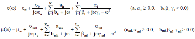
where:
ε∞ is the static conductivity (ε∞ ≥ 0.0),
ε∞ is the infinite frequency relative permittivity (ε∞ ≥ 1.0),
μ∞ is the infinite frequency relative permeability (μ∞ ≥ 1.0),
σm0 is the static magnetic conductivity (σm0 ≥ 0.0),
ak and bk are first order electric material expansion coefficients (ak ≥ 0.0 and bk ≥ 0.0),
α1, β1, and γ1 are second order electric material expansion coefficients (α1 ≥ 0.0 and β1γl ≥ 0.0),
amk and bmk are first order magnetic material expansion coefficients (amk ≥ 0.0 and bmk ≥ 0.0),
αm1, βm1, and γm1 are second order magnetic material expansion coefficients (αm1 ≥ 0.0 and γm1 ≥ 0.0),
ω is the angular frequency.
Note the section below, Defining frequency dependent materials, on curve fitting when defining frequency dependent materials. Failure to fit a curve to the data will cause the frequency dependent material to work incorrectly.
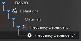
Assigning frequency dependent materials
Check to make sure all of the relevant structures in the Structure Tree are checked to make them visible.
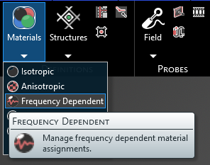
Click Materials
 within the Definitions section under the EMA3D tab in the ribbon.
Click
 Frequency Dependent in the drop-down list.
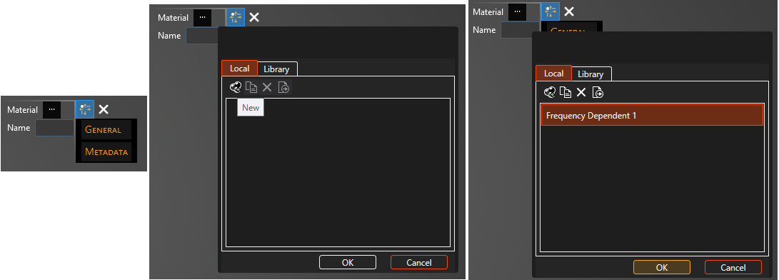
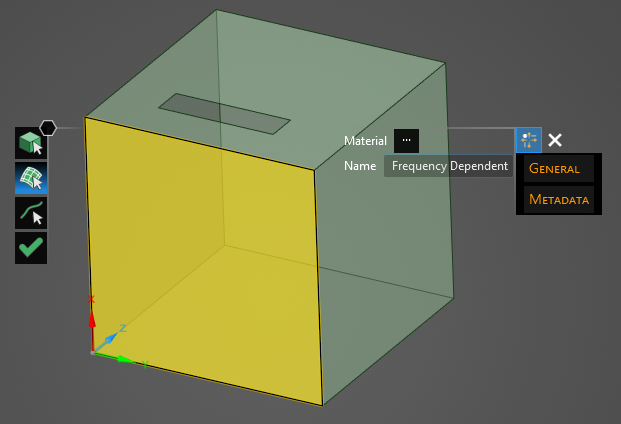
In the Properties panel select the ellipsis to the right of Material. A new window will appear. In the pop-up window, under the Local tab, select New
 .
.
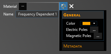
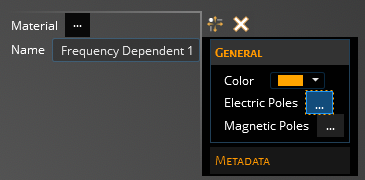
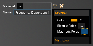
Double click to select the first definition in the list Frequency Dependent. Click General to view and change any property values. Select a material property to see its definition. A list of material properties and their definitions is provided at the bottom of this page. The color is in A, R, G, B format and choosing an A between 0 (most transparent) and 255 (opaque) can make the color and mesh semi-transparent. The next section has instructions for setting the electric and magnetic pole coefficients.
Click on the appropriate selection tool (i.e., body
 , surface
 , or line
 ) tool in the top left of the model window to restrict the assignment definition.
To assign material properties, either select the geometric entity in the model window or in the Structure Tree.
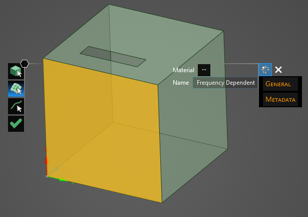
The selected surfaces will be recolored in the model window.
To hide the color and revert to the original, more transparent view, uncheck the check box next to Isotropic under the Definitions node in the Simulation Tree or uncheck Definitions to hide all materials.
Repeat the above steps to assign as many materials as desired.
Click
 to complete the material assignments.
Defining frequency dependent materials
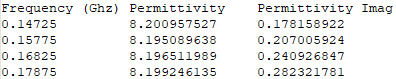
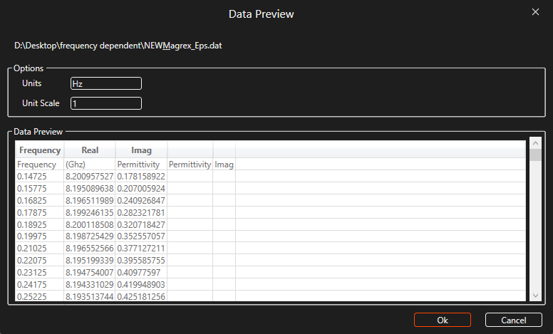
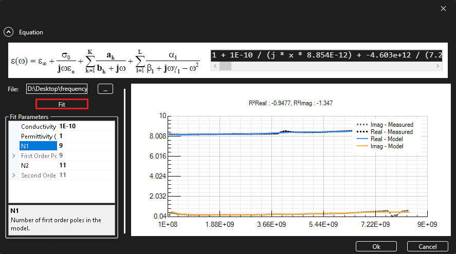
Two text files are required to define frequency dependent materials - one defining the permitivitty and the other defining the permeability. Each file should consist of three columns separated by spaces or commas: the first column is the frequency (units do not matter, they can be set in the GUI wizard), the second column is the real component of the permittivity/permeability, and the third column is the imaginary component of the permittivity/permeability.
To begin defining a frequency dependent material, click on the General box then the ellipsis next to Electric Poles in the Properties Panel.
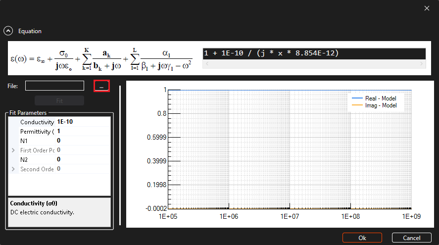
A new pop-up window will appear. In the pop-up window, click the ellipsis next to File.
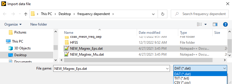
A new pop-up window will appear. In the pop-up window, select the .dat, .txt, or .csv file that corresponds to the permittivity. Click Open.
A new pop-up window will appear. In the pop-up window, change the Units box to match the units in the file. The Unit Scale will update automatically.
Click OK to complete.
A curve must now be fit to the data. Enter the number of first and second order poles next to N1 and N2, respectively. The greater the number of poles the longer it will take to fit the data. Click Fit. The frequency dependent material will only work properly if the curve fitting has been completed.
Once the curve matches to the user's satisfaction, click OK.
Repeat the above steps for the magnetic poles by clicking the ellipsis next to Magnetic Poles in the Properties Panel and repeating the above steps using the file containing the permeability data.
Entry | Meaning |
|---|---|
Material Libraries | Local frequency dependent material definition to assign to the geometry. |
Name | Name of the material. |
Entry | Meaning |
|---|---|
Color | Color to use when rendering the material. |
Electric Poles | Material permittivity model.
|
Magnetic Poles | Material permittivity model.
|
Entry | Meaning |
|---|---|
Part Number | Part number of material (if any). |
Company | Company of material (if any). |
Category | Category of material (if any). |
Abbreviation | Abbreviation of material (if any). |
Description | Description of material (if any). |
Short Name | Short name description of material (if any). |
Long Name | Long name description of material (if any). |
Version | Version of material (if any). |
Other Resources
EMA3D – © 2026 EMA, Inc. Unauthorized use, distribution, or duplication is prohibited.