Animation Window

This section will discuss the creation of the animation window for surface charging output data.

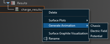
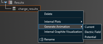
1. Right click the 'charge_results' in the Results section of the simulation tree. This will bring up the pop up menu where you can follow Surface -> Generate Animation to bring up the 3 data options to make an animation for.

   

    

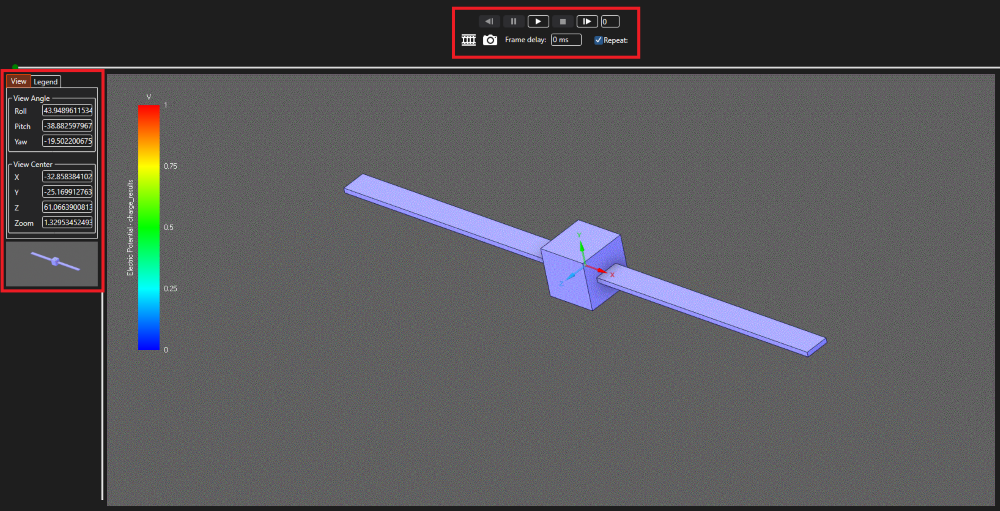
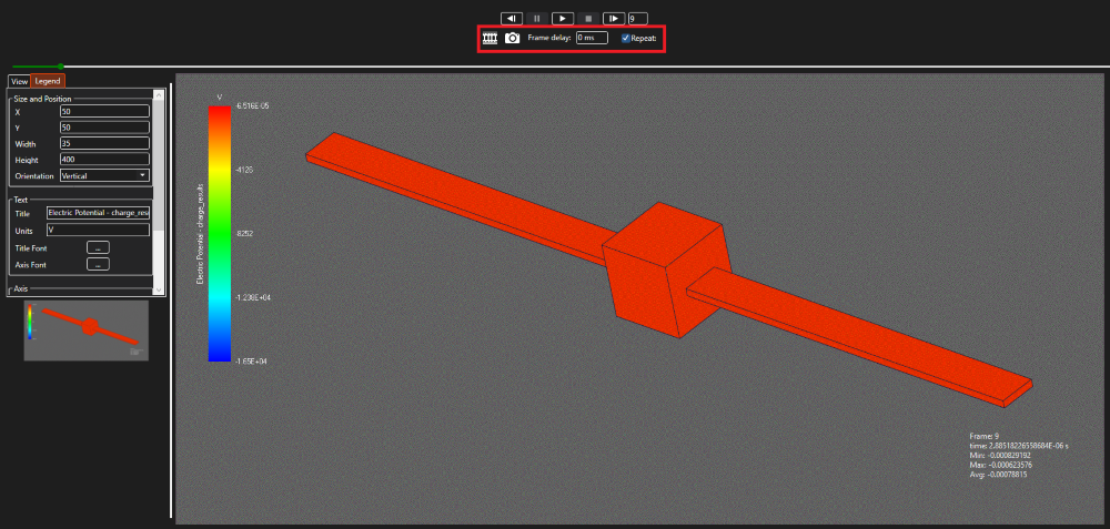
2. Below is an example animation window for the surface potential of a toy satellite. You will see the model in the animation window, the automatically generated legend in the left of the window, animation controls along with export options in the middle top (highlighted below) and lastly there are two tabs on the far left that show parameters for the View (highlighted below) and the Legend.

   

    

3. In order to maneuver the model that appears in the animation window the user has two options. The first option is to adjust the view values in the View tab. The second option is go into the native model window of Discovery and adjust the view. Scrolling the middle mouse wheel zooms in and out on the model. By holding the middle mouse button you can rotate the model around, and doing so while holding Ctrl allows you to pan the model. Keep in mind that if you choose the latter, and keep the animation window open, you will need to press play to see the change in view.

    

4. The animation controls are in the top middle of the window, with basic Previous and Next buttons to skip through time steps, Along with the Pause , Play , and Stop buttons to control the animation. To the right of the Next button, you will see a numbered entry which indicates the time step number the animation is currently at.

    

5. If you press the Play button in the animation window, you will see the time steps running and depending on what you have displayed on your model, be it the materials, meshing cells etc., you should see some coloring of the animation jumbled with the model. At this point it is necessary to have the geometry not fully displayed so that the animation coloring does not interfere. Since the animation window is linked to the Discovery window, the user can modify how the geometry is displayed in Discovery and make it transparent in the animation window.

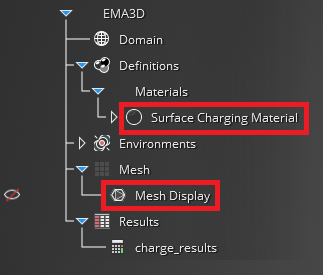
   Make sure the animation is stopped by hitting the Stop button and return to the Discovery window. Within Discovery, go to your Simulation Tree and under Definitions, deselect the Materials to hide the coloring in the model. Likewise, if you have the mesh cells displayed, in the Simulation Tree under Mesh, deselect the Mesh Display and any Mesh Groups you have created.

   

    

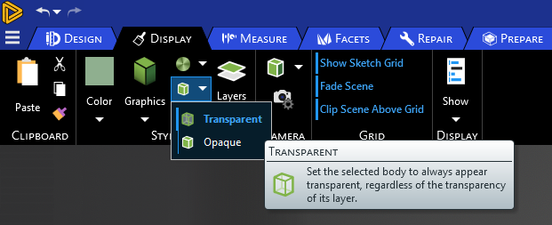
6. Under your Structure Tree, make sure that you have the solid of your model selected. Go to the Display tab of Discovery and within the ribbon in the Style section, you will see a style override button. Select this and select the Transparent option.

   

    

7. Returning now to the animation window and pressing play , you will see the animation run through the time steps defined by the domain without the geometry coloring interfering with the animation coloring.

   Pressing Play puts the animation in 'play mode', where you can only Pause or Stop the animation. While in play mode, you cannot skip through time steps with the Previous or Next buttons. Only when the animation is stopped can the user skip through the steps and manually go through the animation to investigate the changes in values. If the user knows a specific time step they would like to jump to they can type it in the time step entry to the right of the Next button which again can only be done when the simulation is stopped.

   

    

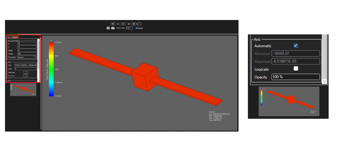
8. The image above has the Legend tab selected of the animation window to show the available options to modify the legend of the animation. Within Size and Position, the X and Y entries allow the user to change the position of the legend within the window, with the Width and Height to modify the legend size. Orientation can be either Vertical or Horizontal.

9. Under Text, the user can change the title of the legend, the units displayed, along with font stylizing of the title and the axis numbering.

10. Under Axis is where the user can customize the legend scaling. The automatic scaling will try to cover between the min and max of the whole simulation. The user can manually adjust the scale if they is interested in just a specific time segment of the simulation, or if they're interested in just a particular material that covers a narrower value range over the simulation time. This is done by first unchecking the Automatic box in the Axis section. This un-greys the Minimum and Maximum entries for the scale, where the user can now use values to are closer to those of interest in specific parts of the simulation. If the values that are displayed over the course of the simulation vary over an extreme scale, you can try using the Logscale option to allow the animation to run through these values more timely. Finally, the Opacity of the animation coloring can be varied, and can help illustrate the backside of the model during the animation.

11. There are exportation options for either the whole animation as a .gif, or images of specific time frame steps. The exportation option buttons are in the middle top of the animation window.

    

     

12. Clicking on the Export Animation button opens up browse window to save your animation as a .gif file. Delays between frames can be added to the .gif with the Frame Delay entry in the animation window. This can be useful if the time steps are really short and there are large changes in the data output. Selecting Repeat in the animation window encodes the .gif to repeat when played.

13. Clicking on the Export Frame button opens up browse window to save your the current frame of the animation as a .png, .jpg, .bmp or .gif file.

This section will discuss the creation of the animation window for internal charging output data.

1. Right click the 'charge_results' in the Results section of the simulation tree. This will bring up the pop up menu where you can follow Internal -> Generate Animation to bring up the 3 data options to make an animation for.

   

    

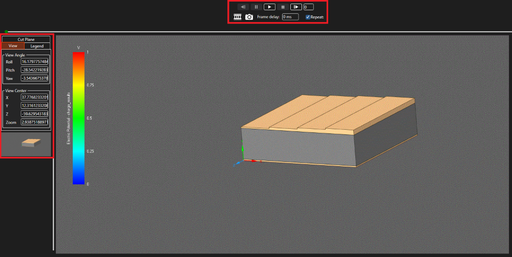
2. Below is an example animation window for the surface potential for the stepped shield example. You will see the model in the animation window, the automatically generated legend in the left of the window, animation controls along with export options in the middle top (highlighted below) and lastly there are three tabs on the far left that show parameters for the View (highlighted below), Legend, and Cut Plane.

   

    

3. Refer to step three of Internal Animation Window for information on viewing.

    

4. The animation controls are in the top middle of the window, with basic Previous and Next buttons to skip through time steps, Along with the Pause , Play , and Stop buttons to control the animation. To the right of the Next button, you will see a numbered entry which indicates the time step number the animation is currently at.

    

5. If you press the Play button in the animation window, you will see the time steps running and depending on what you have displayed on your model, be it the materials, meshing cells etc., you could see some coloring of the animation jumbled with the model. At this point it is necessary to modify what is displayed so that the animation coloring does not get interfered. Since the animation window is linked to the Discovery window, the user can modify how the geometry is displayed in Discovery and make it transparent in the animation window.

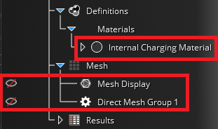
   Make sure the animation is stopped by hitting the Stop button and return to the Discovery window. Within Discovery, go to your Simulation Tree and under Definitions, deselect the Materials to hide the coloring in the model. Likewise, if you have the mesh cells displayed, in the Simulation Tree under Mesh, deselect the Mesh Display and any Mesh Groups you have created to hide them.

   

    

6. Under your Structure Tree, make sure that you have all the solids of your model selected. Go to the Display tab of Discovery and within the ribbon in the Style section, you will see a Style Override button. Select this and select the Transparent option.

   

    

7. Returning now to the animation window and pressing Play , you will see the animation run through the time steps defined by the domain without the geometry or materials coloring interfering with the animation coloring.

   Pressing Play puts the animation in 'play mode', where you can only Pause or Stop the animation. While in play mode, you cannot skip through time steps with the Previous or Next buttons. Only when the animation is stopped can the user skip through the steps and manually go through the animation to investigate the changes in values. If the user knows a specific time step they would like to jump to they can type it in the time step entry to the right of the Next button which again can only be done when the simulation is stopped.

    

8. Refer to step eight of Internal Animation Window for information on Size and Position.

    

9. Refer to step nine of Internal Animation Window for information on Text.

    

10. Refer to step ten of Internal Animation Window for information on Axis.

    If the values that are displayed over the course of the simulation vary over an extreme scale, you can try using the Logscale option to allow the animation to run through these values more timely.

    Finally, the Opacity of the animation coloring can be varied, and can help illustrate the backside of the model during the animation.

     

11. Probably the most important tab for an internal animation is the Cut Plane. The animation displays the output data in internal geometry by slicing it with a plane and displaying the value gradients on the plane. Where the user locates this plane and orientation is done within the Cut Plane tab of the animation window. The example below is from the stepped shield tutorial, with the cut plane on the X-axis, placed halfway into the model.

    

     

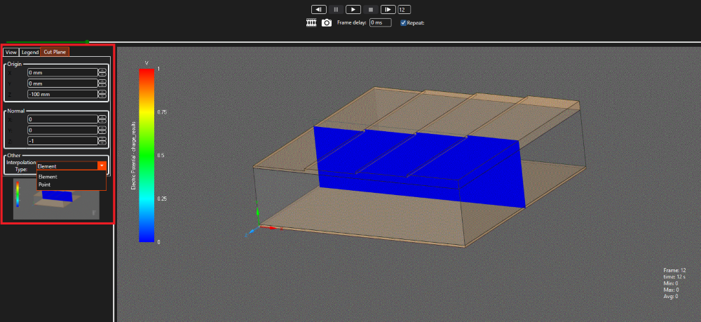
12. Within the Cut Plane tab, there is an Origin section, a Normal section and an Other section.

    • Origin- Sets the plane displacement from the origin along the X, Y, and Z axis.

    • Normal- Dictates the orientation of the plane relative to the X, Y, and Z axis.

    • Other- Determines handling of the gradient interpolation either between cell Elements or Points. Point tends to make the gradient a bit smoother.