Localized

As stated at the top of Section 5.6 only the first four localized sources are discussed below. The localized sources for the thin wires and the cylindrical conductors are defined in Section 5.8.1 and Section 5.8.2.

If a source file is specified, then it can be used by any number of localized sources. All source files are in ASCII format with two columns of data as shown below:

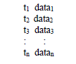
where: ti is the time in seconds, and data is the source value in MKSA units.

EMA3D® analysis always begins at time zero, with all electromagnetic fields and sources set to zero. Therefore, the first record in all source files must start out with: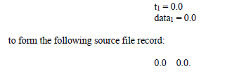

Failure to begin a file with zeros results in an error message and EMA3D program termination.

The times, ti, do not have to correspond with the simulation times associated with the finite difference time step. If the finite difference simulation time falls between time values in the source file, then the required source value will be computed by linear interpolation between neighboring values in the source file. Therefore, if a linear ramp-like source is desired, only two data file records are necessary – the initial record (0.0 0.0) and the final record (t1 data1). If the last time record, tn, in the source file is less than the final time of the finite difference simulation, then source values of zero will be used until the computation is complete.

There are four keywords associated with the first four localized sources. These keywords are provided below.

• ELECTRIC CURRENT DENSITY SOURCE

• MAGNETIC CURRENT DENSITY SOURCE

• ELECTRIC FIELD SOURCE

• MAGNETIC FIELD SOURCE

Each of these four keywords are discussed in separate subsections below.

The utilization of electric current density sources is one of the more common methods of driving a finite difference model. For example, a line of electric current density sources is usually devised to simulate a lightning current channel or an electric arc. Electric current density sources can exist within any material in EMA3D including linear backgrounds, nonlinear backgrounds, isotropic materials, composite materials, anisotropic materials, frequency dependent materials, PEC materials or PMC materials. However, if electric current density sources are located within PEC materials, then a warning message will result. The consequence of doing this is the removal of all effects associated with the source.

The locations of electric current density sources are specified by identifying geometry where the sources are to be applied, with additional descriptors provided to specify how the source is to be applied. This may require construction of source geometry in addition to the model geometry already present.

The source geometry required depends upon the current density source desired. If a current channel is desired, then a geometric line, or perhaps several lines, should be constructed to represent the current channel. Analogously, a geometric surface, or many surfaces, can be constructed to represent a sheet of current.

The information within the associated source file, or that associated with a predetermined analytic waveform, should be considered a current and not a current density. The current values are appropriately synthesized to yield the proper current density within the respective material and for the respective finite difference spatial increments. Thus, to model a first return lightning strike, only the current values of the first return stroke (Lightning Current Component A), need be considered.

Magnetic current density sources can exist within any material in EMA3D including linear backgrounds, nonlinear backgrounds, isotropic materials, anisotropic materials, frequency dependent materials, PEC materials, and PMC materials. However, if magnetic current density sources are located within PMC materials, then a warning message will result. The consequence of doing this is the removal of all effects associated with the source.

The locations of magnetic current density sources are specified by identifying geometry where the source is to be applied, with additional descriptors provided to specify how the source is to be applied. This may require construction of source geometry in addition to the model geometry already present.

The source geometry required depends upon the current density source desired. If a current channel is desired, then a geometric line, or perhaps several lines, should be constructed to represent the current channel. Analogously, a geometric surface, or many surfaces, can be constructed to represent a sheet of current.

The information within the associated source file, or that associated with a predetermined analytic waveform, should be considered a magnetic current and not a current density. The current values are appropriately synthesized to yield the proper current density within the respective material and for the respective finite difference spatial increments.

Electric field sources can exist within any material. However, this is trivial since the implementation of this type of source is achieved by merely setting the specified electric field to a specified multiple of the value in the source file. This is equivalent to using an infinite impedance voltage source. If an electric field source is embedded within PEC material, that is, surrounded by PEC material, then a warning message will result. The consequence of doing this is the removal of the effects of the source. However, if the sources exist on, and parallel to, the surface of PEC material, then it can be used as a driving source. This method is discussed for the two-step seam analysis procedure discussed below.

The locations of electric field sources are specified by identifying geometry where the source is to be applied, with additional descriptors provided to specify how the source is to be applied. This may require construction of source geometry in addition to the model geometry already present.

The source geometry required depends upon the field source desired. If a channel of fields is desired, then a geometric line, or perhaps several lines, should be constructed to represent the channel. Analogously, a geometric surface, or many surfaces, can be constructed to represent a sheet of fields.

EMA3D has the capability of directly modeling seams in various materials (see Section 5.9). However, there is a two-step process using electric field sources that may prove useful in some cases. The configuration is shown in Figure 5.6.2.3.1. The two-step process consists of an exterior model and an interior model. The first step involves the exterior model, in which the seam is absent, where current density (h-fields) values are recorded at the location where the seam is desired. These current density values are for current flowing across the seam at locations along the entire length of the seam. Typically, the wall containing the seam is metallic or PEC. The second step involves the interior model where the electric field sources at the location of the seam, on the surface of the seam material, are used to drive the interior problem. As discussed above, electric field sources can exist on the surface of PEC or metallic structures and can be used as drivers. The necessary electric field sources are computed using the seam impedance approach below.

Seams are usually characterized by an impedance. The seam impedance typically has a resistive, R, and an inductive, L, component. Typical seam resistance values exist within the range from 1.0 μΩ to 1.0 mΩ-m and typical seam inductance values exist within the range from 100 pf-m to 10 nf-m with the former values characterizing a good seam. For seam analysis, the assumption is made that the voltage, V(t), across the seam is given by:

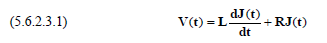
where, J, is the exterior current density at the seam location. Therefore, if the seam exterior surface current densities are computed with the exterior model, then the seam voltages can be calculated. This must be done outside of EMA3D.

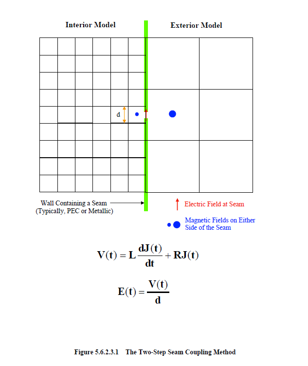
The resultant interior fields across the seam are given by:

where, d, is the interior finite difference spatial increment across the seam. This also must be done outside of EMA3D.

As shown in Figure 5.6.2.3.1, the resolution of the interior model does not have to be the same as the exterior model. Typically, the interior model has a more fine mesh. The absence of the seam in the exterior model means that this two-step process is weakly-coupled or one-way. That is, the interior problem does not affect the exterior responses.

Magnetic field sources can exist within any material. However, this is trivial since the implementation of this type of source is achieved by merely setting the specified magnetic field to a specified multiple of the value in the source file. This is equivalent to using an infinite impedance magnetic voltage source. If a magnetic field source is embedded within PMC material, that is, surrounded by PMC material, then a warning message will result. The consequence of doing this is the removal of the effects of the source. However, if the sources exist on and parallel to the surface of PMC materials then it can be used as a driving source.

The locations of magnetic field sources are specified by identifying geometry where the source is to be applied, with additional descriptors provided to specify how the source is to be applied. This may require construction of source geometry in addition to the model geometry already present.

The source geometry required depends upon the field source desired. If a channel of fields is desired, then a geometric line, or perhaps several lines, should be constructed to represent the channel. Analogously, a geometric surface, or many surfaces, can be constructed to represent a sheet of fields.