Extended

There are four keywords associated with extended sources. These keywords are provided below.

• PLANE WAVE SOURCE

• BOX IN SOURCE (Used with Subgrids)

• BOX OUT SOURCE (Used with Subgrids)

• GAMMA SOURCE

Each of these keywords are discussed in separate subsections.

The plane wave source algorithm generates a plane wave within a specified closed rectilinear volume. A plane wave is useful when computing the electromagnetic responses from a source that exist at a great distance from the object being modeled. The plane wave is manufactured by computing electric and magnetic current density values on the equivalent surface of the rectilinear volume. These are then injected into the equivalent surface electric and magnetic fields in the proper manner, and with the proper retardation time, to generate a plane wave within the surface boundary. The plane wave is confined to the equivalent surface volume. Scattered fields, however, will propagate through the surface and escape to the outer boundaries of the problem space. This feature, in conjunction with the EMA3D Far Field algorithm, enables the computation of scattered fields created by plane wave excitation and, therefore, can be used for such phenomena as radar cross-section computations.

Only one plane wave source may be utilized. If more than one is specified within the EMA3D input file, the last one read will be implemented – all others will be ignored. In addition, a plane wave source cannot be implemented with a gamma source.

The plane wave source waveform is supplied using a data file or a predetermined analytic waveform. The data file or the analytic waveform defines the plane wave electric field value as a function of time.

There are several aspects associated with plane waves that require consideration. These are discussed immediately below, followed by instructions on plane wave specification.

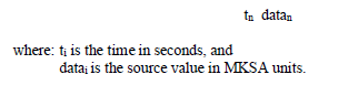
If a data file is used, then this file must be unique and cannot be shared by any other sources. The source information supplied in the data file must be in ASCII format with two columns of data as shown below:

EMA3D analysis always begins at time zero, with all electromagnetic fields and sources set to zero. Therefore, the first record in all source files must start out with:

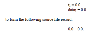
Failure to begin a file with zeros results in an error message and EMA3D program termination.

The times, ti, do not have to correspond with the simulation times associated with the finite difference time step. If the finite difference simulation time falls between time values in the source file, then the required source value will be computed by linear interpolation between neighboring values in the source file. Therefore, if a linear ramp-like source is desired, only two data file records are necessary – the initial record (0.0 0.0) and the final record (t1 data1)

If the last time record, tn, in the source file is less than the final time of the finite difference simulation, then source values of zero will be used until the computation is complete.

If a predetermined analytic waveform is desired, then the source symbols (GAUSS, DGAUSS, etc) must be used (see Section 5.6.4).

When specifying a plane wave, the spatial extent of the equivalent surface must be defined. The equivalent surface must be contained within the finite difference problem space. If this is violated, an error message will be issued, and the program terminated.

When specifying a plane wave, the orientation parameters that specify the incident direction and the electric field polarization must be defined. The plane wave incident direction (propagation vector) and electric field polarization are both characterized by a polar angle and an azimuthal angle. The polar angle is defined as the angle from the positive z-coordinate axis. The azimuthal angle is defined as the angle from the positive x-coordinate axis to the perpendicular projection of the vector onto the xy coordinate plane. There are thus four angles required to specify the plane wave orientation. The electric field vector and the propagation vector must be orthogonal or an error message will result in EMA3D and the program will terminate. If a PEC or a lossy ground plane is present, then the propagation vector must have a component that points into the ground. For a grazing angle, this component can be as small as 10-3 degrees. If θ is the polar angle of the propagation vector, ϕ is the corresponding azimuthal angle, α is the polar angle of the electric field vector, and β is the corresponding azimuthal angle, then the allowable ranges of these parameters are:

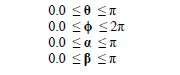
Any values outside of these ranges will result in an error message in EMA3D and program termination.

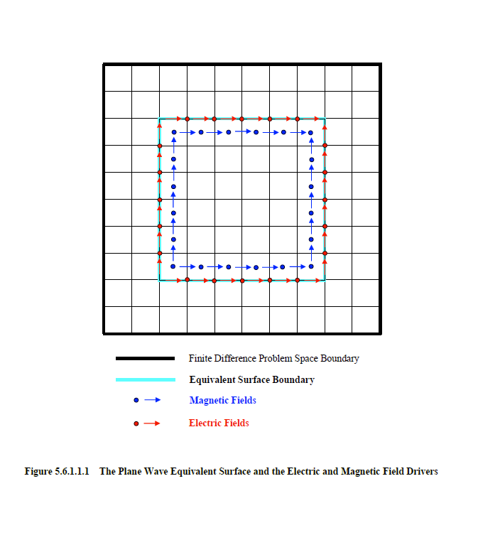
A two-dimensional slice through a three-dimensional finite difference problem space containing a plane wave equivalent surface is shown in Figure 5.6.1.1.1. The problem space, in the plane of the page, has dimensions 10 by 10. The equivalent surface has dimensions 6 by 6. Superimposed are the electric and magnetic fields in which the current density values are injected to generate the plane wave. Therefore, the equivalent surface boundary extends, in depth, one half of a finite difference cell into the surface volume.

The current density values at the locations of the electric and magnetic fields must be properly timed to generate the plane wave. The retardation times are dependent upon the electromagnetic speed of propagation. There is thus an inherent medium associated with an equivalent surface from which the propagation speed is derived. The inherent medium is determined in EMA3D by inspecting all materials that penetrate the plane wave equivalent surface, including background materials. A material penetrates the surface if it exists within the half-cell depth discussed above. In the absence of a ground plane (discussed below), the inherent medium is determined by the material constituting the majority of surface penetrations. If a ground plane is detected, the inherent medium is determined by the material constituting a majority of surface penetrations on the side of the ground from which the plane wave originates – the origination direction being determined by the plane wave propagation vector discussed above. The inherent medium must be both electrically and magnetically nonconductive. It can possess any permittivity and permeability value greater than or equal to the respective vacuum values. However, if a lossy ground is present, then the permeability must be that of a vacuum. In most cases, the inherent medium is nothing more than the implicitly programmed vacuum background.

Any material that penetrates the plane wave equivalent surface boundary with electromagnetic parameters different from that of the inherent medium, ground plane excluded, disrupts the timing and degrades the nature of the generated plane wave. Therefore, any material penetration results in a warning message in EMA3D. The program may be continued, but effects of the penetration should be understood and perhaps monitored. This only applies to materials that penetrate the surface boundary, not to those that exist within.

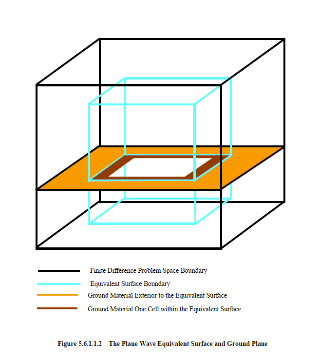
The presence of a ground plane is confirmed within EMA3D if a material, with a given set of electromagnetic parameter values different from that of neighboring materials (including the inherent background), extends from at least one cell within the equivalent surface, on all four sides, to the problem space boundary, as depicted in Figure 5.6.1.1.2. The algorithms within EMA3D check for a one-cell penetration only. However, the material can extend deeper into the equivalent surface volume, even forming a continuous plane. Most ground planes specified are continuous planes. If the ground plane is not continuous, as depicted in Figure 5.6.1.1.2, then there is a hole in the ground plane. This is a perfectly legitimate configuration and could be used to simulate many geometries such as a pit in the ground (PEC or lossy) or an aperture through a PEC ground plane.

If two perpendicular ground planes are detected, an error message will result, and the program will terminate. If two parallel planes are detected, the one closest to the side of the problem space from which the plane wave originates will be the one selected. If a perfectly conducting ground is detected, then the spatial extent of the equivalent surface will be automatically modified within EMA3D to contact the ground. A PEC boundary condition can also be specified on one side of the problem space to simulate a perfectly conducting ground.

The ground plane material can be perfectly conducting, lossy, or dielectric. If σ, ε, μ, and σm are the conductivity, permittivity, permeability, and the magnetic conductivity values of the inherent medium and σg, εg, μg, and σgm are the corresponding values of the ground plane, then the permissible values are listed below.

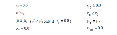
If any of these conditions are violated, an error message will result and EMA3D will terminate.

A two-dimensional configuration can be specified in EMA3D. If a two-dimensional configuration exists, in conjunction with a plane wave, then the propagation vector must lie within the two-dimensional plane. There are two possible two-dimensional specifications consisting of the normal electric field and the normal magnetic field configurations (see Section 5.3.2). If the normal magnetic field two-dimensional configuration is specified, then the electric field polarization vector must lie within the two-dimensional plane. If the normal electric field configuration is specified, then the electric field polarization vector must be perpendicular to the two-dimensional plane. If any of these conditions are violated, an error message will result and EMA3D will terminate.

There are several types of boundary conditions available within EMA3D. These were discussed in Section 5.5 and listed for convenience below.

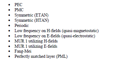
As discussed above, the plane wave is confined to the equivalent surface volume. The scattered fields, however, propagate through the surface and escape to the outer boundaries of the problem space. If PEC or PMC boundaries are used, except for PEC on one problem space side to simulate a perfectly conducting ground, then a physically nonsensical solution will result when the scattered fields are reflected off the boundaries. This is because the plane wave, presumably of near infinite extent, will enter the confines of the equivalent surface unimpeded by the perfectly conducting boundaries. For this reason, if PEC or PMC boundary conditions are specified (PEC ground plane excepted) with a plane wave source, a warning message will be issued.

If a symmetric boundary is specified, then the plane wave propagation vector must be parallel to the boundary or boundaries of symmetry. This also applies to periodic boundaries. Violating this condition, results in an error message and EMA3D program termination. In addition, for either symmetric or periodic boundary conditions, the equivalent surface bounds must physically contact the problem space boundary where these conditions are employed. Otherwise, a physically nonsensical solution will result when the scattered fields encounter the boundary. If contact is not made, a warning message will result in EMA3D.

For the other boundary conditions, the equivalent surface should not be placed within a certain number of finite difference cells from the problem space boundary. The number of cells depends upon the particular boundary condition. The reason for this is some of these boundary conditions use fields a few cells within the finite difference problem space to compute the boundary fields. If the equivalent surface invades this realm, then the boundary condition will use both incident and scattered field components to compute a boundary field that should only be computed with scattered fields. The number of cells from the boundary is dependent upon the boundary condition employed. For each boundary condition, the number of cells is provided below.

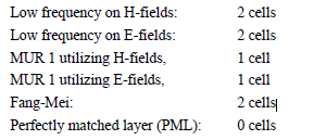
Placing the equivalent surface closer than the minimal cell distance above will elicit a warning message in EMA3D.

Even though the minimal number of cells varies with the boundary condition used, it is recommended that a two-cell distance be kept for all of the boundary conditions, except symmetric, periodic, or PEC boundaries of course. This will enable a change of boundary condition without having to modify the plane wave equivalent surface bounds.

The plane wave equivalent surface can be locked in place, if desired, or it can be set for modification. Modification, if selected, will be enacted for certain boundary conditions. Modification for PEC, symmetric, or periodic boundary conditions consist of equivalent surface adjustment to touch the offending boundary. If open boundary conditions are employed, then modification to 2 cells within the problem space bounds will be enacted.

EMA3D has the capability of storing electric and magnetic fields on a specified rectilinear surface. These fields are then used to create equivalent electric and magnetic current sources to drive another numerical simulation. The intent of this procedure is to provide a mechanism to drive a numerical problem of finer spatial resolution. The finer resolution problem is contained within the geometry of the coarse problem space. The fields are first stored in the simulation of the coarse problem. In the simulation of the finer resolution problem these fields are synthesized and interpolated to provide equivalent sources to drive the interior problem of much finer resolution. This procedure is thus a two-step process. The first step involves the storage of the electric and magnetic fields. The second step involves the use of these fields to create the electric and magnetic current driving sources.

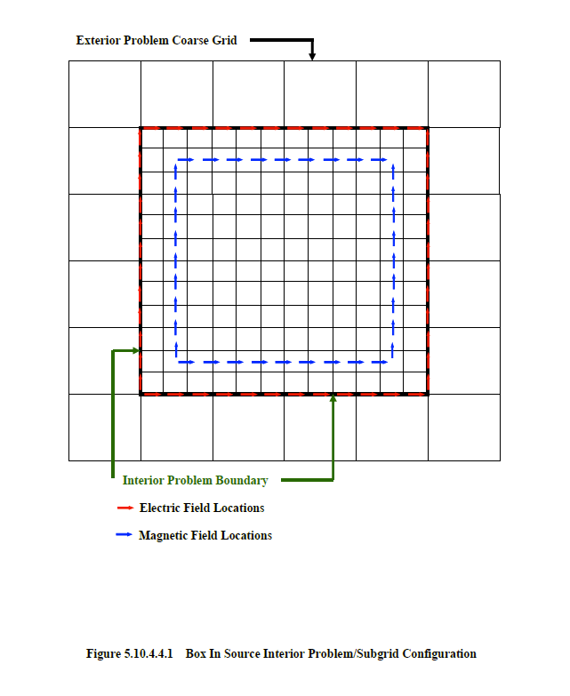
The first step in this procedure is associated with the Box In Probe (see Box In Probe discussion in Section 5.10.4.1). Implementation of the Box In Probe results in the generation of a file containing the coarse problem electric and magnetic fields on a specified rectilinear surface (see Figure 5.10.4.1.1). This will be termed the exterior problem. The second step involves the Box In Source. This utility uses the fields from the Box In Probe to drive another finite difference problem. This is termed the interior problem. The communication from the exterior problem to the interior problem is thus one-way or weakly-coupled. The electromagnetic response of the interior problem does not impact the driving sources and therefore does not affect the exterior problem.

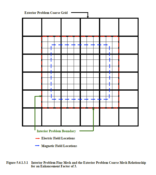
This Box In feature was principally devised to drive an interior problem with a finer spatial resolution then that of the exterior problem. It would make little sense to drive an interior problem of the same spatial resolution. This has already been achieved by the exterior problem. The relationship between the coarse mesh exterior problem and the fine mesh interior problem is depicted in the two-dimensional representation of Figure 5.6.1.2.1. This figure should be compared to Figure 5.10.4.1.1. In Figure 5.6.1.2.1, the size of the fine mesh cells is a factor of three smaller than those of the exterior coarse grid problem, in both coordinate directions constituting the plane of the page. This factor will be termed the resolution enhancement factor. For the Box In Source the resolution enhancement factor must be greater than or equal to 1.

To provide the proper electric and magnetic current density sources, to be used as drivers for the interior problem, requires interpolation of the exterior field quantities stored in the output file of the Box In Probe. The degree of interpolation, and the location of injection, depends upon the enhancement factor. The red arrows in Figure 5.6.1.2.1 indicate the location of the electric fields where the electric current density values are injected. These exist at the same location as the exterior electric fields of Figure 5.10.4.1.1. To properly align the magnetic fields, however, requires the selection of the magnetic fields at the locations indicated by the blue arrows in Figure 5.10.4.1.1. In both cases, electric and magnetic field interpolation of exterior problem fields, in both space and time, are required to get the interior fields.

The electric and magnetic fields of the exterior coarse mesh problem are recorded by specifying a Box In Probe. During the simulation of the exterior problem the enhancement factor is unknown. However, the mesh information and the Box In Probe equivalent surface information are recorded in the Box In Probe output file. The enhancement factor is realized when the information in the Box In Probe is read during execution of the Box In Source facility.

When specifying a Box In Source, it is best to avoid material penetrations of the box in surface. This includes any penetrations by more than one background. The interpolation scheme used is less accurate in regions closest to material penetrations. Therefore, the rectilinear surfaces associated with both the Box In Source and the Box In Probe, should be defined to avoid penetrations as much as possible. If any portion of the box in equivalent surface is exterior to the finite difference problem space bounds, an error message will result, and the program will terminate.

To implement a Box In Source requires specification of the rectilinear surface and the Box In Probe file name. It is essential that the dimensions of the Box In Source rectilinear surface and the Box In Probe rectilinear surface be identical. It is not essential, of course, that the two occupy the same physical location in space – that is, possess the same coordinates with respect to some common origin.

The Box Out Source is similar to the Box In Source but is executed in the opposite direction. As stated in Section 5.6.1.2, EMA3D has the capability of storing electric and magnetic fields on a specified rectilinear surface. These fields are then used to create equivalent electric and magnetic current sources to drive another numerical simulation. The intent of this procedure is to provide a mechanism to drive a numerical problem possessing a more coarse spatial resolution. The fields are first stored in a problem with a fine spatial resolution. In a separate simulation problem, these fields are synthesized and used to provide equivalent sources to drive a problem with a coarse spatial resolution. The fine resolution problem thus exists within the geometry of the coarse resolution problem. This procedure is thus a two-step process. The first step involves the storage of the electric and magnetic fields. The second step involves the use of these fields to create the electric and magnetic current driving sources.

The first step in this procedure is associated with the Box Out Probe (see Box Out Probe discussion in Section 5.10.4.2). Implementation of the Box Out Probe results in the generation of a file containing the electric and magnetic fields on a specified rectilinear surface (see Figure 5.10.4.2.1). This will be termed the interior problem. The second step involves the Box Out Source. This utility uses the fields from the Box Out Probe to drive another finite difference problem. This is termed the exterior problem. The communication from the interior problem to the exterior problem is thus one-way or weakly-coupled. The electromagnetic response of the exterior problem does not impact the driving sources and therefore does not affect the interior problem.

This particular feature was principally devised to drive an exterior problem with a more coarse spatial resolution then the interior problem. The relationship between the coarse mesh exterior problem and the fine mesh interior problem is depicted in the two-dimensional representation of Figure 5.6.1.3.1. This figure should be compared to the Box Out Probe depiction in Figure 5.10.4.2.1. In Figure 5.6.1.3.1, the size of the interior problem fine mesh cells is a factor of three smaller than those of the exterior coarse grid problem, in both coordinate directions constituting the plane of the page. This factor will be termed the resolution enhancement factor. For the Box Out Source the resolution enhancement factor must be greater than or equal to 1.

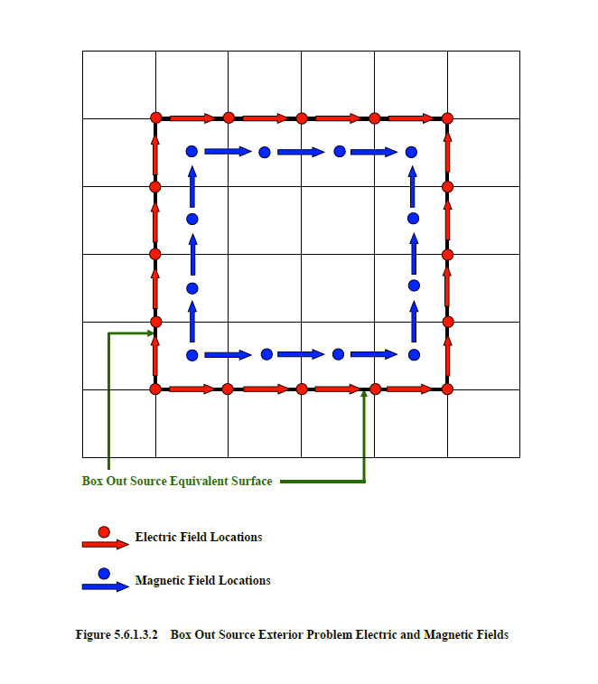
To provide the proper electric and magnetic current density sources, to be used as drivers in the exterior coarse mesh problem of the Box Out Source, requires averaging of the fine mesh interior field quantities computed during the simulation associated with the Box Out Probe. The red arrows in Figure 5.6.1.3.1 indicate the location of the Box Out Probe simulation electric fields and the blue arrows the location of the magnetic fields. These fields are averaged in both space and time to produce the exterior problem coarse mesh fields seen in Figure 5.6.1.3.2. To avoid creation of excessively large files containing numerous fine mesh fields, these fields are averaged in space and time during the simulation of the interior fine mesh problem and recorded in the Box Out Probe output file. To accomplish this requires foreknowledge of the desired Box Out Source enhancement factor during execution of the Box Out Probe facility. The Box Out Probe mesh information, enhancement factor, and equivalent surface information are recorded in the Box Out Probe output file.

When specifying a Box Out Source, it is best to avoid material penetrations of the Box Out Probe and the Box Out Source equivalent surface. This includes any penetrations by more than one background. The interpolation scheme used is less accurate in regions closest to material penetrations. Therefore, the equivalent surfaces should be defined to avoid penetrations as much as possible. If any portion of the Box Out Source equivalent surface is exterior to the finite difference problem space bounds, an error message will result in EMA3D and the program will terminate.

To implement a Box Out Source requires specification of the rectilinear surface and the Box Out Probe file name. It is essential that the dimensions of the Box Out Source rectilinear surface and the Box Out Probe rectilinear surface be identical. It is not essential, of course, that the two occupy the same physical location in space – that is, possess the same coordinates with respect to some common origin.

Gamma ray sources are used primarily for nuclear source region electromagnetic pulse (SREMP) coupling computations, which include system generated electromagnetic pulse (SGEMP) and internal electromagnetic pulse (IEMP) phenomena. The nuclear source region exists in the neighborhood of a nuclear explosion, where other effects such as the shock wave and thermal radiation are present. During a nuclear explosion, gamma rays interact with air molecules to produce a flux of Compton electrons that generate the electromagnetic pulse. In addition to the electromagnetic pulse, the source region contains source currents and ionizing gamma rays.

The implementation of gamma sources requires a data file containing the waveform of the gamma dose rate. The gamma dose rate is then used to calculate the ionization rate. The gamma dose rate needs to be in rads/second. (Note: 1.0 Grays/second = 100.0 rads/second)

There are two user-defined parameters associated with the gamma ray source. These concern the gamma source incident direction polar angle and the associated azimuthal angle. The polar angle is defined as the angle from the positive z-coordinate axis. The azimuthal angle is defined as the angle from the positive x-coordinate axis to the perpendicular projection of the vector onto the xy coordinate plane. If, θ, is the polar angle and, ϕ, is the azimuthal angle, then the allowable ranges of these parameters are:

Any values outside of these ranges will result in an error message and program termination. The gamma source file must be unique and cannot be shared by other sources.