Isotropic

For PEC materials, all interior electric fields are zero. In many cases, highly conductive metals such as silver, copper, aluminum, and iron, can be modeled as perfectly conducting. An exception would arise if the mechanism of diffusion through the material were deemed important and significant. If this is the case, then isotropic materials or composite materials should be used.

For PMC and PEC materials, both interior magnetic and electric fields are zero. However, there is a different material boundary condition. For PMC materials there are nonzero normal magnetic fields and nonzero tangential electric fields. For PEC materials, there are nonzero normal electric fields and nonzero tangential magnetic fields.

The nonmetal isotropic material refers to all materials that can be characterized by defining a conductivity (σ), a permittivity (ε), a permeability (μ), and a magnetic conductivity (σm). For most materials, the permeability is equal to the vacuum value (1.257e-6 henries/meter) while the magnetic conductivity is zero. All isotropic materials must possess permittivity and permeability values greater than or equal to the respective vacuum values. Conductivities must not be negative. The range of acceptable electromagnetic parameter values are shown below.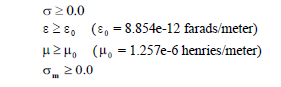

Assigning values outside of this range will result in an error message and program termination.

When isotropic nonmetal materials overlap, the electromagnetic parameters for all isotropic materials within the overlap region are averaged, resulting in only one isotropic material within that particular region.

To accurately model isotropic nonmetal materials, in a general sense, all frequencies within the materials should be adequately resolved. This implies a finite difference mesh cell size capable of resolving the smallest wavelength (highest frequency) of interest. To resolve a particular frequency requires ten cells per wavelength. In isotropic materials, the wavelengths are a function of the electromagnetic parameters – these parameters being: the conductivity, the permittivity, the permeability, and the magnetic conductivity. As the values of these parameters increase, the wavelengths within the materials decrease.

Resolving the wavelengths can be rather prohibitive, from a computer resource perspective, due to the small cells required to resolve the higher frequencies. This is especially pronounced for conductive materials. However, there are procedures that allow one to avoid the resolution requirement, in many cases, without impacting computational accuracy to any significant degree. As a matter of fact, these procedures, in many cases, are quite accurate. When addressing such procedures, it is best to discuss insulating and conducting materials separately. Only applications to electric materials are discussed. Those for magnetic materials follow similarly

Insulating Materials - Frequency Resolution

The wavelength, λ, within insulting materials (zero conductivity) is given by the following formula.

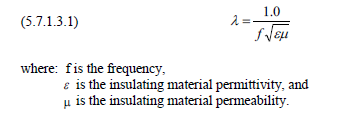
To resolve the wavelength computed by the above formula, in a finite difference computation, requires 10 mesh cells per wavelength. Therefore, the cell dimension, dg, is given by the following equation.

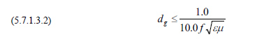
Some examples of the maximum cell dimension (in meter units), computed for a range of frequencies and relative permittivity values, are provided in the table below.

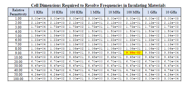
The first line in the table above is identical to the finite difference cell dimension required to resolve the indicated frequency within a vacuum.

Insulating Materials - Surface Modeling using Low Frequency Approximation

If coupling through an insulating material surface with a thickness less than the finite difference cell dimension, in the normal direction to the surface, is of interest, then the low frequency approximation may be used. The low frequency approximation increases the accuracy of the simulation results for thin insulating surfaces. An accuracy assessment is provided in the EMA3D Validation Manual.

The technique is implemented by adjusting the insulating material conductivity according to Equation (5.7.1.3.3) below.

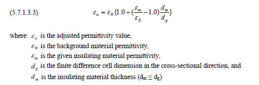
The permittivity adjustment constitutes a scaling with respect to the cell dimension in the cross-sectional direction. The reason for the permittivity adjustment is as follows. A thin material, when meshed, assumes a thickness of the mesh dimension, dg, in the cross-sectional direction. If the permittivity of the meshed material, εg, were assigned the given material permittivity, εm, and dg ≠ dm, then the result would be a material with a different thickness possessing the same permittivity value. The nature of electromagnetic interaction with the material depends upon the permittivity and the material thickness.

Lossy Materials - Frequency Resolution

For conducting materials, the expression for the wavelength is more complicated than for insulating materials. However, if

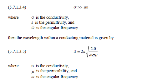
The condition of Equation (5.7.1.3.4) is met in a vast majority of cases. To resolve the smallest wavelength of interest requires ten finite difference mesh cells. Therefore, the cell dimension, dg, is given by:

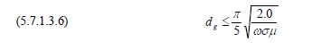
The maximum cell dimension required to resolve several different frequencies in materials with various conductivity values are shown in the table below.

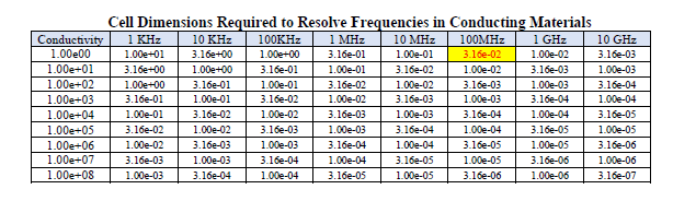
Inspection of the table reveals a somewhat restrictive nature of the ten cell per smallest wavelength resolution requirement. For example, if a material possessing a conductivity of 1.0 mhos/meter were present and located at positions throughout the model, then to resolve frequencies up to 100 MHz would require a mesh size of 3.16E-2 meters (the highlighted red font value in the table). For a problem space of 30 × 30 × 30 meter problem a mesh size of 3.16E-2 meters implies a problem space size of approximately 950 by 950 by 950 mesh cells resulting in a memory requirement of about 21 gigabytes (single precision). This size of a problem is not too restrictive but the presence of materials with higher conductivities may prove otherwise. However, resolving the maximum frequency in lossy material may not always be necessary, as discussed below.

Resolving the highest frequency with ten finite difference cells of dimension, dg, is a brute force method that does not have to be implemented in many modeling situations. When addressing mesh sizes for conducting materials, it is advantageous to think in terms of the thickness of the material being modeled, dm, the cell dimension, dg, and the associated skin depth, dk.

If Equation (5.7.1.3.4) is satisfied, then the skin depth, dk, for electric materials, is given by the following equation.

The skin depth decreases as the frequency increases. The skin depth values (in meter units), computed for a range of frequencies and conductivity values, are provided in the table below.

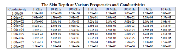
It is important to note that if the condition of Equation (5.7.1.3.4) is satisfied, then the ten cell resolution requirement of Equation (5.7.1.3.6) results in adequate resolution of the skin depth. The skin depth can be thought of as an upper bound of dg. If this is the case, then the highest frequency is resolved by 6.3 finite difference cells.

Lossy Material Modeling - Low Frequency Approximation

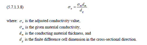
The lossy material low frequency approximation involves an adjustment of the associated conductivity value. The conductivity adjustment involves a scaling with respect to the ratio of the material thickness to the selected mesh increment. The scaling is given by the equation below.

The result of the conductivity adjustment is to define a new material that possesses an equal resistance to that of the given lossy material. This provides an accurate technique at low frequencies. This is often used to model materials excited by low frequency phenomena such as lightning.

The accuracy of the lossy material low frequency approximation is addressed in the EMA3D validation Manual.

Lossy Material Modeling - Methods

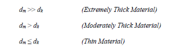
When selecting a mesh size for lossy isotropic materials it is instructive to think in terms of material thickness and three thickness regimes. These regimes are defined as Extremely Thick Materials, Moderately Thick Materials, and Thin Materials. If dk is the skin depth of the smallest wavelength of interest and dm is the material thickness, then the three regimes are as defined below.

If an Extremely Thick Material is being modeled, then diffusion through that material is negligible and it is no longer necessary to resolve the skin depth (and the associated ten cell per wavelength requirement). In this case the cell dimension does not have to be selected based upon the skin depth or the material thickness and can be based upon other geometric resolution considerations of the model. Such applications are particularly applicable when modeling highly conductive materials such as aluminum. In many cases, including those concerning aerospace vehicles with metallic skins, the skin thickness is much greater than the associated metal material skin depth at the highest frequency of interest.

If a Moderately Thick Material is being modeled, then three different modeling methods are available. The first is to use the same considerations applied to an Extremely Thick Materials and model directly with no modification of geometric or material parameter values. The accuracy of this method should be assessed. The second method is to select a cell size that is greater than the material thickness and define the isotropic material as a composite material (see Section 8.4.1). This method, however, may not be possible due to other model geometric resolution requirements. The third method is to use a low frequency approximation (see below) and gauge the accuracy.

If a Thin Material is being modeled, then two different modeling methods are available. The first method is to select a cell size that is greater than the material thickness and define the isotropic material as a composite material (see Section 8.4.1). For Thin Materials this method may be more realizable than for Moderately Thick Materials, but could also be limited by other model geometric resolution considerations. The second method is to use a low frequency approximation. The low frequency approximation was discussed above.

Using the following definitions:

• dm is the conducting material thickness,

• dg is the finite difference cell dimension in the cross-sectional direction, and

• dk is the wavelength, in the conducting material, of the highest frequency of interest.

The three methods discussed above are outlined below:

1. Extremely Thick Materials ( dm >> dk )

   • Select dg based on general resolution requirements of inherent model

   • Directly model lossy material with no alterations of material parameters

   • Can model lossy material as PEC in many situations

2. Moderately Thick Materials ( dm > dk )

   • Method 1

     1. Model as an Extremely Thick Material

     2. Assess accuracy of applied method

   • Method 2

     1. Select dg > dm

     2. Use Composite Material Algorithm

   • Method 3

     1. Select dg based on general resolution requirements of inherent model

     2. Use Lossy Material Low Frequency Approximation

     3. Assess accuracy

3. Thin Materials ( dg ≤ dk)

   • Method 1

     1. Select dg > dm

     2. Use Composite Material Algorithm

   • Method 2

     1. Select dg based on general resolution of inherent model

     2. Use Lossy Material Low Frequency Approximation

Composite materials are isotropic materials with a user-defined thickness that is less than or equal to the finite difference cell dimension in the cross-sectional direction. Composite materials are not finite difference materials, in the normal sense, but the implementation of a mathematical algorithm designed to simulate the presence of a thin isotropic, frequency independent material, of considerable conductivity, such as the 10,000 mhos/meter value associated with carbon fiber composites – thus the name, “composite materials”. Considerable conductivity implies:

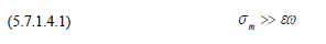
where, ω, is the highest angular frequency present in the computation. This usually implies the highest frequency resolvable by the finite difference mesh. Failure to adhere to the above criteria may result in numerical inaccuracies or numerical instabilities. A two order-of-magnitude cushion is recommended.

The composites formalism allows incorporation of thin, lossy material surfaces with thicknesses too small to be directly resolved. Composite materials are characterized by user-supplied values of a conductivity (σ), a permittivity (ε), a permeability (μ), a magnetic conductivity ( σm) and the material thickness ( dc). All composite materials must possess permittivity values equal to the respective vacuum values and a magnetic conductivity value equal to zero, as specified below:

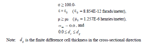
Assigning permittivity, permeability, and magnetic conductivity values different than those specified above, will result in warning messages with all values being reset to the corresponding correct values. Assigning a negative conductivity value, a negative material thickness, or a material thickness greater than the respective cross-sectional finite difference cell thickness, will result in an error message and program termination. Assigning a thickness of zero will elicit a warning message with the composite being effectively removed from the problem.

If composite materials overlap, the electromagnetic parameters of all composite materials within the overlap region are averaged, resulting in only one composite material in that region with the resultant averaged parameter values. The composite thicknesses, however, are not averaged. Overlapping composite materials each with a different thickness will result in an error message and program termination.

Magnetic absorber surfaces are isotropic materials with a user-defined thickness that is less than or equal to the finite difference cell dimension in the cross-sectional direction. Magnetic absorber surfaces are not finite difference materials, in the normal sense, but the implementation of a mathematical algorithm designed to simulate the presence of a thin isotropic surfaces with magnetic absorber properties.

The magnetic absorber formalism allows incorporation of thin, lossy material surfaces with thicknesses too small to be directly resolved. Magnetic absorber materials are characterized by user-supplied values of a conductivity (σ), a permittivity (ε), a permeability (μ), a magnetic conductivity ( σm) and the material thickness ( da). The range of acceptable magnetic absorber material parameters is shown below.

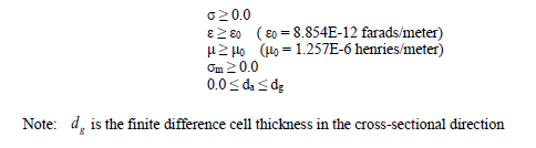
Assigning conductivity, permittivity, permeability, magnetic conductivity, and a material thickness values outside of the ranges specified above, will result in error messages and program termination. Assigning a thickness of zero will elicit a warning message with the magnetic absorber being effectively removed from the problem.

If magnetic absorber surfaces overlap, the electromagnetic parameters of all magnetic absorber surfaces within the overlap region are averaged, resulting in only one magnetic absorber surface in that region with the resultant averaged parameter values. The thicknesses, however, are not averaged. Overlapping magnetic absorber materials, each with a different thickness, will result in an error message and program termination.