MHARNESS Cables

The MHARNESS® solver is a multi-conductor, multi-branched, multi-shield cable solver. Like EMA3D®, MHARNESS requires an input file containing all geometry and cable definitions. The format of the MHARNESS input file, including all cable descriptions and definitions, is addressed in the MHARNESS User Manual.

There are two keywords associated with MHARNESS cables. These keywords are provided below.

Each of these keywords is discussed in separate subsections below.

The MHARNESS INFILE keyword is used to define the name of MHARNESS input file. The format of this file is provided in the MHARNESS User Manual.

Within MHARNESS are entities called segments. An MHARNESS segment is a set of parallel conductors, each possessing a constant cylindrical cross-section and a constant inter-conductor geometric relationship throughout the length of the segment. The inherent conductors interact through impedance matrices (capacitance, inductance, and conductance). A dielectric jacket may be defined on any conductor within the segment. Each segment is therefore defined with a constant cross-section throughout the entire length. A segment conductor may consist of a shield or a wire. A shield may contain other conductors within. These interior conductors, whether additional shields or wires, constitute a different MHARNESS segment. All conductors on the inside of a shield are not directly exposed to the EMA3D electromagnetic environment because these are shielded. Only conductors that are not shielded are exposed to the EMA3D electromagnetic environment. These conductors, whether shields or wires, constitute an ‘exposed’ segment.

Only the exposed MHARNESS segment names and associated mesh information is provided in the EMA3D input file. All other cable information, included nonexposed segments, segment composition, impedances, terminations, and junctions, are defined within the MHARNESS input file. Like cylindrical conductors, only one MHARNESS cable can exist at any one location. If this is violated, then an error message will result and EMA3D terminated.

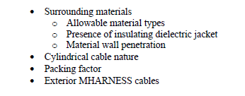
The many features of MHARNESS are presented in the MHARNESS User Manual. Only those features concerned with the definition and placement of the cable within the three-dimensional problem space of EMA3D are discussed here. These features are listed below.

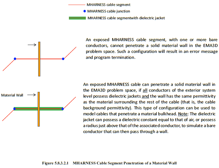
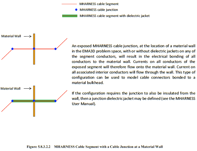
An exposed MHARNESS cable segment must exist entirely within a linear background or within an insulting isotropic material, or a lossy isotropic material. Immersion within other EMA3D materials is not allowed. Furthermore, an MHARNESS cable segment must exist entirely within the same material, except at the cable endpoints. Different materials at the endpoints allows for the termination of cables to such structures as ground planes or bulkheads. However, if a dielectric jacket is employed on all conductors within an exposed cable segment, then the cable can exist within allowable isotropic materials that possess different conductivities. The permittivity, nevertheless, must still be the same along the entire length of the cable, except at the cable endpoints. The configurations and ramifications of passing an MHARNESS cable segment through a material wall in EMA3D are portrayed and described in Figure 5.8.3.2.1 and Figure 5.8.3.2.2.

An MHARNESS cable segment within EMA3D is automatically assigned the radius of a cylinder that physically contains all the conductors and corresponding dielectric jackets associated with that segment. The algorithms used to simulate an MHARNESS segment within the EMA3D problem space are designed to simulate cylindrical cable bundles and not necessarily such entities as ribbon cables. An MHARNESS cable segment associated with such a ribbon cable will be assigned a radius of a cylinder that contains all the ribbon conductors. The electric fields within the described cylinder will be used to drive the ribbon and the currents on each of the ribbon conductors will be injected into all the electric fields within the cylinder volume. If non-cylindrical configurations are modeled, then the effect on simulation accuracy should be assessed.

MHARNESS cable segments are associated with sets of geometric lines in the EMA3D GUI. However, a geometric line is a one-dimensional entity. As long as the radius is small (much less than the finite difference cell dimension in the cross-sectional direction), the MHARNESS segment is represented by a single meshed line. However, as the radius increases, the segment will encounter neighboring cells. This results in a three-dimensional character with associated consequences not particularly obvious by inspection of the relevant geometric line.

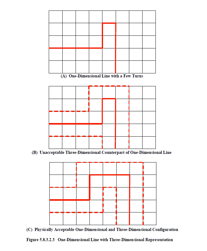
There are certain topologies that a one-dimensional line can assume that are not possible in a three-dimensional sense (i.e. when the cable radius increases). One such configuration is shown in Figure 5.8.3.2.3A. Within this figure is a line, depicted as solid red, that is superimposed upon a finite difference cubic mesh. The line makes a few turns and then continues on. If the radius was to increase, thereby expanding into neighboring cells, then the corresponding three-dimensional geometric representation would be impossible to achieve, as shown in Figure 5.8.3.2.3B. The conductor would expand into itself resulting in a geometric configuration that would be physically impossible. If this were to occur in the defining problem, then an error message would be produced in EMA3D and the program terminated. A more realizable situation is shown in Figure 5.8.3.2.3C. Expanding the one-dimensional line in this figure into neighboring cells results in a physically realizable three-dimensional configuration.

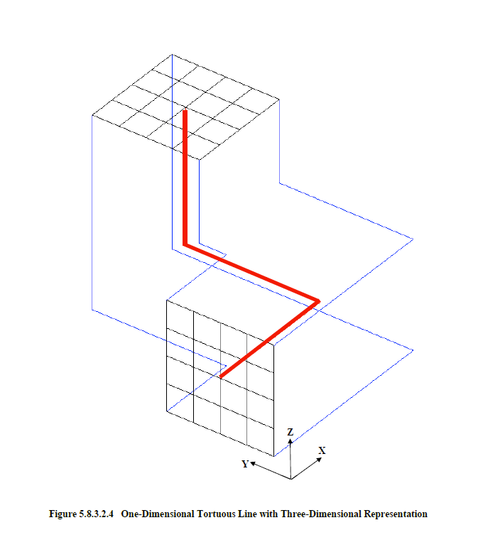
Another common topology is shown in Figure 5.8.3.2.4. Here a conductor line, colored red, starts in the x-coordinate direction, turns to the y-coordinate direction, and then to the z-coordinate direction. A superimposed mesh is shown at both ends of the conductor line. Assume this conductor were to be assigned a radius causing it to expand until it was bounded, in a cross-sectional sense, by the blue lines. If the conductor line was modified so that the length of the line segment in the y-coordinate direction was decreased to a value less than the conductor diameter, then the line segment in the z-direction would move against the segment in the x-direction. This would crimp the conductor in a physically unrealizable manner. If this were to occur in the defining problem, then an error message would be produced in EMA3D and the program terminated.

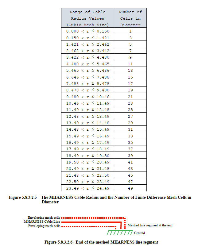
To assess the resultant topology requires knowledge of the finite difference cells enveloped as a function of the assigned conductor radius. MHARNESS can only be used when a cubic mesh is employed. This is to effect proper connection among all meshed cells. For this reason, a radius can be expressed in terms of the cubic mesh size. The range of cable radii and the resultant number of required cells in diameter is shown in the table of Figure 5.8.3.2.5.

On the ends of all MHARNESS cable segments are placed PEC end caps that span across all enveloped cells. If the cable depicted in Figure 5.8.3.2.4 was the entire conductor, from beginning to end, then the mesh observed on both ends would be PEC material. This is done to conductively bond all finite difference cells within the line at either end, as required. The end caps can be observed using the proper keywords in the Structure Probe (see Section 5.10.5.1), the Picture Probe (see Section 5.10.5.2), and the Slice Probe (see Section 5.10.5.3).

The mesh of the line at the end of all MHARNESS segments must be in one coordinate direction only, for a distance at least one cell longer than the associated cable segment radius. This is required to effect proper topology and proper attachment to materials, as shown in Figure 5.8.3.2.6.

MHARNESS cables can possess radii that expand over many finite difference cells. For radii with values much smaller than the inherent finite difference cell dimension, the cable is totally contained, in a cross-sectional sense, within a single cell. However, as the radius increases, the cable will expand into neighboring cells thereby requiring more cross-sectional cells for accurate modeling. If the cable is contained within a confined physical space, then this expansion may prove cumbersome if extensive geometry modifications are required to accommodate the cable. It may prove beneficial to have the option of packing the cable into a tighter space, even if such packing impacts accuracy (to an acceptable degree) of the numerical simulation.

Within EMA3D is a packing factor variable that allows this activity to be done. The packing factor ranges in value from “0.3” to “0.9”. The default value is “0.4”. However, the value of, “0.3” provides the greatest degree of accuracy. As the packing factor increases, the maximum allowable cable radius before expansion into neighboring cells, increases. A table of the packing factor and the maximum associated radius in provided below.

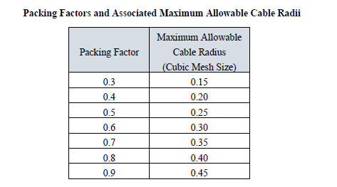
As an example, assume that a cable with a radius of 0.32 times the value of the finite difference cubic cell exists. Furthermore, assume that this cable exists in a confined space consisting of only one finite difference cell in diameter. Inspection of table in Figure 9.5 shows that this cable would require 3 finite difference cells in diameter to effect proper simulation. This is because a value of 0.32 exceeds the maximum allowable radius of 0.15 that is required to fit into a single cell. The maximum value of 0.15 is associated with the default packing factor value of 0.3. However, if a packing factor of 0.7 was specified, then the maximum allowable radius would be 0.35, according to the table above, and the cable could then be packed into a single finite difference cell, in the cross-sectional direction.

There is, however, consequences of increasing the packing factor value. As this value increases, the accuracy is reduced and the possibility of a numerical instability arises. For a packing factor of “0.9”, an error upwards of 10%, or higher, is possible. However, as mentioned above, it may prove useful to trade numerical accuracy, to an acceptable degree of course, for the ability to tightly pack the cable into confined physical spaces. The algorithms within EMA3D are designed to detect if a numerical instability might arise, and if so, to render advice concerning actions that might be taken to avoid such an occurrence. See the EMA3D Validation Manual for a full assessment of packing factor impacts.

MHARNESS cables can exit the EMA3D finite difference problem space. However, a cable junction must exist at the problem space boundary, as show in Figure 5.8.3.2.7 below. When utilizing such a configuration care should be taken to inspect the impact of cable impedance mismatches, and associated reflections, that may be present at the problem space boundary. To construct such an exterior cable requires no geometry or definitions within the EMA3D problem space or within the EMA3D input file.

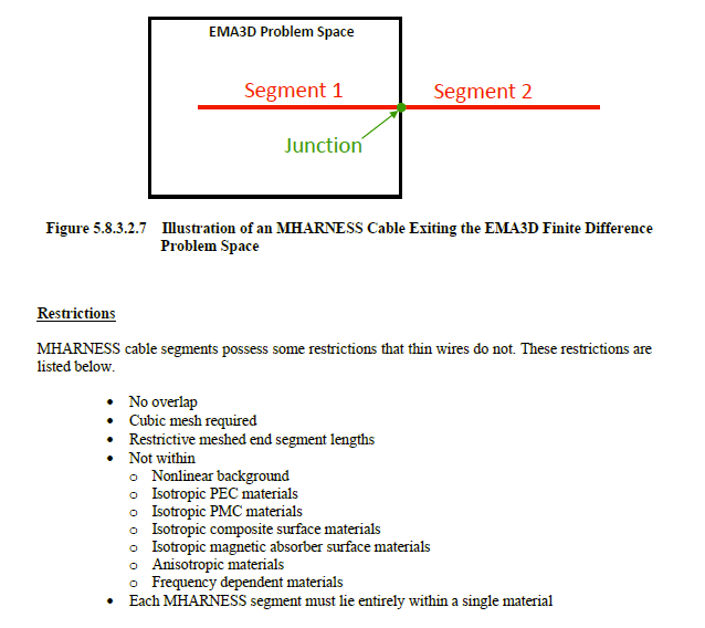
Failure to adhere to these will produce an error message within EMA3D and program termination. The first three topics were discussed above. In addition, MHARNESS cables cannot exist with certain materials. These materials can exist in the finite difference problem space, however, the MHARNESS cable must not penetrate these. If this situation occurs, an error message will be produced and the program terminated. Each individual MHARNESS segment must exist entirely within a single material. Failure to adhere to this will produce an error message in EMA3D and program termination.