Boundary Conditions

The concept of a boundary condition was introduced in Chapter 3 and further discussed in Section 4.1. There is only one keyword associated with boundary conditions. This keyword is listed below:

• BOUNDARY CONDITION

There are eleven different boundary conditions programmed into EMA3D®. Some possess advantages and provide more accurate answers in some situations and less accurate answers in others. Some require greater distances from any scattering objects, or sources, to provide accurate results. Greater distances increase the size of the finite difference problem space.

The eleven boundary conditions can be divided into three groups: exact, quasistatic, and open. The three groups, and the associated boundary conditions within each group, are listed below.

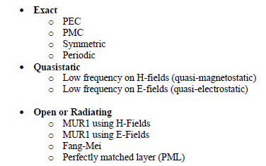
The exact boundary conditions are so termed because the exact values of the boundary fields are known. The quasi-static boundary conditions are those designed for quasi-static situations. The open boundary conditions are designed to simulate an endless extension of the background media, thereby reducing, or eliminating, reflections at the boundary. In EMA3D, a different boundary condition can be specified on each of the six problem space boundaries.

Each boundary condition group is discussed in separate sections below.

In this section exact boundary conditions are discussed. These boundary conditions consist of

• PEC

• PMC

• Symmetric

• Periodic

Each of these exact boundary conditions are discussed in separate subsections below.

PEC boundaries are an exact boundary condition and are implemented by setting all tangential electric fields on designated problem space boundaries to zero. PEC boundaries are useful when the model constructed is within a PEC enclosure, in close proximity to a PEC wall, or on a PEC ground plane. PEC boundaries can be used to simulate a PEC ground plane when the Plane Wave Source is implemented. PEC boundaries are the default condition. If this is the desired boundary condition, then no further action is necessary.

PMC boundaries are an exact boundary condition and are implemented by setting all tangential magnetic fields on plane surfaces one-half-cell outside of the designated problem space boundaries to zero. The magnetic fields are zeroed one-half-cell outside to preserve the integrity of the geometry within the problem space.

Symmetric boundaries are an exact boundary condition that perfectly reflects the geometry, structures, and materials, within the finite difference problem space, across a designated problem space boundary. The utilization of symmetry, if present, is always beneficial because it reduces computation times and memory requirements. For two-fold symmetry, the memory (i.e. the problem space size) and the computation time is reduced by a factor of two, thereby increasing the computational efficiency by a factor of two. For four-fold symmetry, the memory and computation time is reduced by a factor of four thereby increasing the computational efficiency by a factor of four. There are no limitations in EMA3D concerning symmetric boundaries. Any material, geometry, thin wire, cylindrical conductor, MHARNESS cable, thin gap, seam etc., in any configuration, can penetrate or exist on a symmetric boundary.

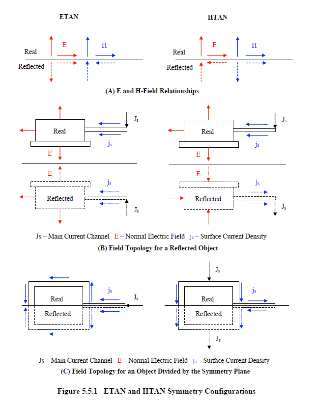
There are two types of symmetries available in EMA3D. These symmetry types are termed, ETAN and HTAN. For both types, the geometry is perfectly reflected while the field topology, as depicted in Figure 5.5.1.3.1A, is quite different. The dashed arrows in the figure represent the fields associated with the reflected geometry. The ETAN symmetry is so termed because the tangential electric fields on either side of the symmetry boundary are equal. For HTAN symmetry, the tangential H-fields on either side of the boundary are equal. Confusion often results when trying to determine which type of symmetry to specify. Some examples are provided that may aid in this endeavor.

The first example is shown in Figure 5.5.1.3.1B. In this figure an object is depicted that appears to resemble a crude type of military tank. There is both the real object and a reflected counterpart. The counterpart is portrayed by a dashed outline. The reflection occurs across a boundary employing a symmetric boundary condition. The real object does not touch the symmetry boundary and has a current channel, Js, attached at the end of the appendage. The resultant field topology, when implementing ETAN or HTAN symmetries, can be seen in the two drawings.

The field topology for an object divided by a symmetry plane is shown in Figure 5.5.1.3.1C. The first drawing portrays a current channel on the symmetric boundary and attached to the appendage. This is an acceptable configuration for the ETAN boundary because the tangential boundary magnetic fields resulting from the current channel are equal and opposite on either side of the boundary, as required by inspection of Figure 5.5.1.3.1A. Implementing an HTAN symmetric boundary for this case would result in a nonsensical configuration. This is because the tangential boundary magnetic fields, under HTAN symmetry, would be set equal in magnitude and direction across the symmetric boundary. However, the current channel and appendage would possess magnetic fields, on either side, that are equal in magnitude but opposite in direction. Implementing an HTAN symmetry for this configuration would prevent a natural flow of current.

The second drawing in Figure 5.5.1.3.1C shows a current channel attached to the side of the object. Implementation of the HTAN boundary results in the field topology shown. If the ETAN boundary were used instead, the reflected current channel would be reversed resulting in two current channels depositing the same sign of charge on the object from each side. This is an acceptable configuration and may be modeled. When invoking symmetry, examine the drawings of Figure 5.5.1.3.1 to aid in the proper selection of the ETAN or HTAN type.

Inspection of the field topology for the ETAN and HTAN boundary condition, may lead to the conclusion that each is identical to the PMC and PEC boundary condition, respectively. In some situations, this may be the case. However, there are differences in implementation. It is best to use the symmetry conditions when symmetries exist, and to use perfectly conducting boundaries when a PEC or a PMC material exists.

Periodic boundaries are an exact boundary condition that can be employed when a repeating geometry is present. Since all geometries are finite, a periodic boundary represents an approximation. However, the approximation can be quite accurate in some cases. An example where a periodic boundary might be employed is the case involving electromagnetic energy coupling to a large antenna array consisting of many identical elements. To model the entire array with the necessary resolution required for each individual element, may prove prohibitive from a budgetary, scheduling, or computer resource perspective. However, modeling a single antenna element with periodic boundaries is much more efficient. The response of the single element can be synthesized (scaled, combined, etc.) to simulate the response of the entire array. In addition, a single element model can possess substantially greater resolution. Periodic boundary conditions may be assigned to any problem space boundary but must always exist on opposite boundaries to produce periodicity.