Open

In this section open boundary conditions are discussed. These boundary conditions consist of:

• MUR1 using H-Fields

• MUR1 using E-Fields

• Fang-Mei

• Perfectly matched layer (PML)

Each of these exact boundary conditions are discussed in separate subsections below.

The Mur 1 boundary condition operated on H-fields is an absorbing or radiating boundary condition. This Mur 1 boundary condition is the oldest radiating boundary algorithm in EMA3D® and may be the least accurate. However, this boundary condition performs well, relatively speaking, when PEC and lossy materials penetrate the boundaries.

The Mur 1 boundary condition operated on E-fields is an absorbing or radiating boundary condition. This Mur 1 boundary condition is the oldest radiating boundary algorithm in EMA3D and may be the least accurate. However, this boundary condition performs well, relatively speaking, when PEC and lossy materials penetrate the boundaries.

The Fang-Mei condition is an absorbing boundary condition that is an enhancement of MUR 1. Fang-Mei boundaries utilize some correction factors to improve the accuracy of the MUR 1 algorithm.

The PML boundary condition is an absorbing boundary condition that is very accurate, but at the same time, computationally intensive. The PML condition requires substantial amounts of computer memory to employ. The procedure for PML involves surrounding the finite difference problem space with layers of absorbing material. The more layers used, the better the solution. However, as the number of layers increases, the amount of required computer memory along with the computation time increases. The thickness of a layer is equal to the mesh cell dimension that borders the finite difference problem space where the boundary condition is employed.

The implementation of PML requires three user-supplied parameters. These parameters are:

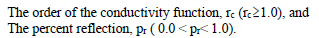
The layers of absorbing material possess nonzero electric and magnetic conductivities. The order of the conductivity function specifies how the conductivity increases from the front to the back layer, where the back layer is always terminated by a PEC surface. Large differences in the conductivity from one finite difference cell to another, within the PML layers, results in numerical reflections. Therefore, if the order is large, then the conductivity varies slowly within the front layers and rapidly increases towards the back layers. If the order is small, then the conductivity increases quickly in the front layers and less so towards the back. If more layers are used then the conductivity will automatically vary more slowly, but this has a large impact on computer resources. The order of the conductivity function must be greater than 1.0. A value assigned outside of this range will result in an error message in EMA3D and program termination.

The percent reflection specifies the amount of electromagnetic energy reflected back into the numerical problem space. Ideally, the value to select is zero. However, making this value too small also results in numerical reflections. The percent reflection should be greater than 0.0 and less than 1.0. A value assigned outside of this range will result in an error message in EMA3D and program termination.

Experimentation has revealed the following values to yield the best results in nearly all situations:

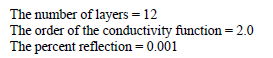
These are the default values used by EMA3D. These can be modified as desired. If these default values prove undesirable, the first change to make is to increase the number of layers.

When specifying PML boundary conditions on any boundary, all applications must have the same number of layers, the same conductivity order, and the same percent reflection, or an error will result and the program will terminate.

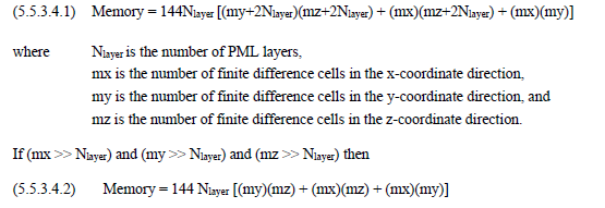
To assess the impact to computer resources when PML boundary conditions are used requires knowledge of the computer memory required by PML. Assuming 4 bytes per variable (single precision), the memory required by PML boundaries is:

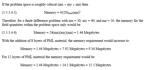
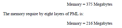
It is evident that PML requires a significant amount of memory that increases substantially as the number of layers is increased. This increase, however, becomes less pronounced as the problem space increases in size. For a roughly cubical problem space (mx my mz) the memory required for the problem space only (see Equation (5.5.3.4.4)) is:

Comparison with Equation (5.5.3.4.3) reveals the memory required by PML to become roughly equivalent with that of the problem space when

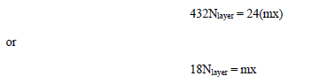
Thus, if Nlayer = 8, then the memory of the problem space exceeds that of PML when, mx, and therefore my and mz, are greater than 144. For mx = my = mz = 250, the memory required by the finite difference problem space is:

PML boundaries should be used if the required memory for implementation falls within the range of allowable computer memory resources and the computation time is not too prohibitive. There are, however, certain situations when PML should not be used. The only materials that should intersect the PML boundaries are background materials with vacuum electromagnetic parameter values. All other materials will impact the accuracy of the result. In addition, electric field sources and current density source should not intersect the boundary. Doing so will result in a build-up of charge on the PML layers.