Surface Charging (CHARGE)

The EMA3D-Charge surface charging module is based on the boundary element method. In this approach, normal electric fields and potentials on elements are written in terms of the charge density on other surface elements using the superposition principle. Matrix relationships are established between the normal electric field and potentials and a time dependent matrix charging equation is the obtained.

To set up our charging equations, we consider each surface element, k, to have a constant charge density, σ_k . Then, the solution to Poisson's equation is given by

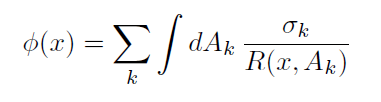
where R is the distance from x to a point on the surface and Φ(x) could be any point in space, but we are interested in solving for Φ(x) on the surfaces.

The above equation can be written in the matrix form:

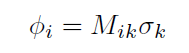
where Φ_i is the potential on a surface element, i, and the repeated index is summed over. A similar approach is used to obtain a matrix equation for the normal electric field at each surface. This allows us to write the charge density on surfaces in terms of the potentials using Gauss's law as well as a capacitive term for non-conductive surfaces. Our resulting matrix equation is of the form:

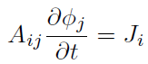
where J_i is the current incident on each surface element, i, and Φ_j is the potential on each surface element, j. In solving this matrix equation, we linearize the currents with respect to the potentials, since the currents in general depend on the potentials.

The surface charging is driven by various current sources which contribute to J_i . In EMA3D-Charge, we support the following currents sources: environmental driven current density from either Maxwellian or Kappa distributions, including the secondary electron yields, backscattered electron yields, and proton induced electron yields, photoemission from sunlight illumination, currents due to surface and volume conduction, triboelectrification, and currents from particle transport include plume and other high energy particle sources.

We can write the current source on surface element,i as:

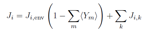
where the summation over k includes all the terms from the contributions mentioned above. Below are two specific example contributions.

For a surface at potential Φ , the current density from a low-energy plasma environment can be written as

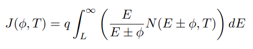
where N is the particle flux at infinity, T is the temperature, E is energy, L is either 0 (for the repelled species) or |Φ| (for the attracted species), and the upper sign is for ions, the lower sign is for electrons.

For a Maxwellian environment, we have

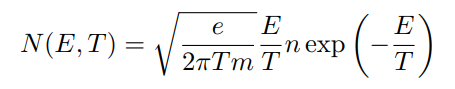
Where n is the number density and m is the particle mass. The current density from this environment can be evaluated analytically.

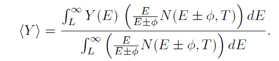
For a surface at potential Φ , the current due to a yield quantity (secondary electron or proton) is given by

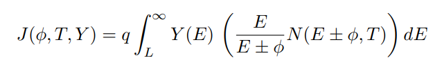
where Y is the electron yield at a given incident energy, E, and