Internal Charging (CHARGE)

The internal charging problem can be simply cast using the continuity equation of electrodynamics:

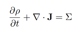
where ρ is charge density, J is current density, and Σ is an external source that generates charge density per unit time.

For the internal charging problem, Σ is the deposition rate of charge due to particle transport in a plasma environment.

Quasi-static formalism

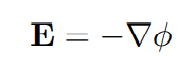
In many applications, the internal charging problem can be adequately treated as a quasi-static problem. If we write the electric field as the gradient of a scalar quantity,

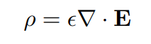
and by recalling the differential form of Gauss’s law,

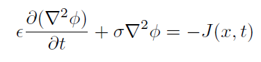
then, the continuity equation becomes,

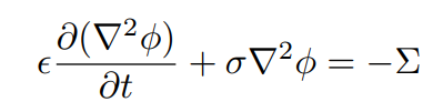
where, J = σ E, and σ is the material conductivity.

Full-wave formalism

For some problems it may be necessary to go beyond the quasi-static approximation to get the full electrodynamic solution, or Full-Wave solution. In this case, the electric field should instead take the form,

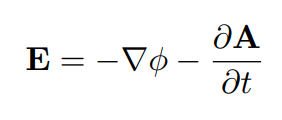
where we have introduced a vector potential, A, which is related to the magnetic field,B = ∇ x A.

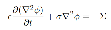
In the Coulomb gauge, ∇·A = 0, and we recover the continuity equation of the quasi-static formalism,

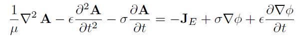
Additionally, the equation for the vector potential A becomes,

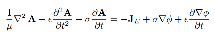
Thus, solving for the quasi-static solution first, allows the right side of equation for the vector potential to be fully known.

Finite-element method (FEM)

EMA3D-Charge uses the finite-element method to solve the above equations. In this approach, we first form a matrix equation on the nodes of a meshed geometry. The specific construction of the matrices depends on the elements of the mesh and user inputs such as material parameters. In order to solve for the system, we convert the element by element matrices into global matrices.

The general matrix equation for each node is of the form,

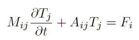
where T_j is the unknown variable, while the matrix A_ij and the vector F_i are known and the indices are the nodal indices.

To construct the continuity equation in matrix form, we need 1) a variational formulation for the spatial information and 2) a differencing approach for the time derivative.

1) Variational formulation

We use the variational formulation with basis functions, γ_i , and the Galerkin method to rewrite the physics equation in the necessary form. For the full wave solution, the matrices needed to solve the scalar potential, Φ , in,

are the following,

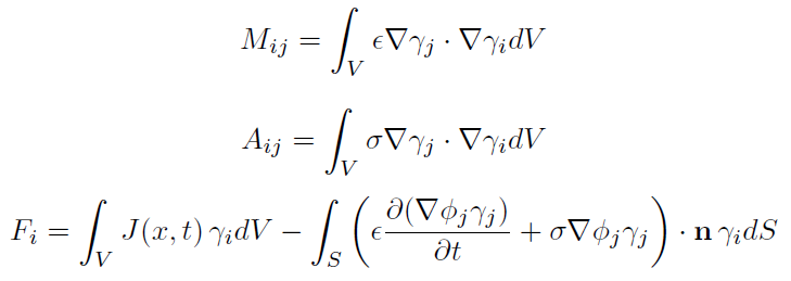
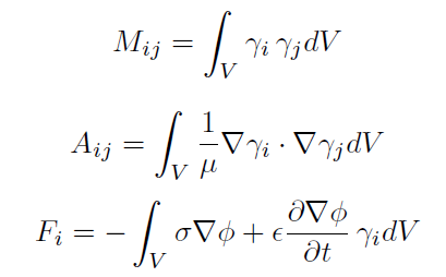
While the matrices to solve the vector potential, A , in,

are the following,

This solution is calculated at the element level and the basis functions are specific to the mesh element type (TR3, QU4, TE4, TE5, PR6, HE8).

2) Backward difference approximation

We can use the backward difference approximation to update the matrix equation at each time step. To solve for the matrices at the next time step, we use the nodal information at the previous and current time steps.

First order backward difference approximation,

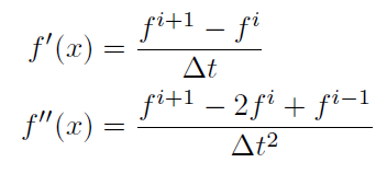
Second order backward difference approximation,

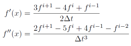
where, fⁱ⁺¹ is the unknown to solve for and the superscripts refer to time step indices.