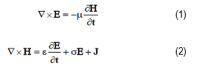
The derivation of the equations used in the FDTD technique for the computation of the electric and
magnetic fields begin with Maxwell’s curl equations. For a linear, homogeneous, isotropic medium,
these equations, in MKSA units, are written as:
where: σ is the conductivity, ε is the permittivity, and μ is the permeability.
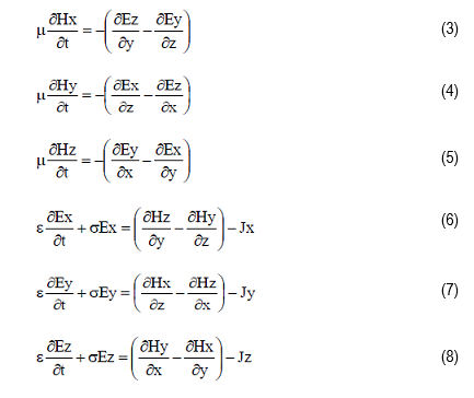
Within these equations is the assumption that the magnetic conductivity is zero. In component form,
the above equations become:
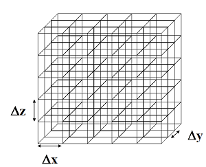
The FDTD method requires a discretization of space with discretization or lattice increments of Δx, Δy, and Δz.
These three values need not be equal or constant throughout space. When space is discretized, as depicted in Figure1,
it is said to be meshed. All objects and materials within the meshed space are also said to be meshed.
The finer the lattice the more closely the meshed object resembles the actual one. Each cell within an object is assigned
material parameters.
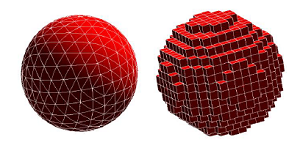
For a sphere consisting of a single material, each of the cells in Figure 2 would possess the same material parameters.
The algorithms in a finite difference solver are tied directly to the lattice. The lattice is made up
of intersecting lines that are parallel to the coordinate axes. A point where lines from the three coordinate
directions intersect is called a lattice point. Any lattice point can be specified by the spatial lattice indices (i,j,k).
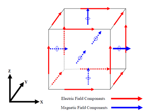
An enlarged view of one particular lattice cell, with superimposed electric and magnetic fields,
is shown in Figure 3.
This cell shows electric fields along the edges of the cell and magnetic fields perpendicular to the cell faces.
The various field components (Ex, Ey, Ez, Hx, Hy, Hz) are staggered throughout the lattice facilitating the use
of an accurate centered-differenced formulation. The locations of the electric and magnetic fields, with respect
to a lattice cell, could just as well be switched by shifting the coordinate origin by half a cell dimension in
each coordinate direction.
However, EMA3D uses the convention of Figure 3. Inspection of this figure, in conjunction with the index terminology
introduced above, shows each field component to be uniquely defined by a single set of three integer indices (i,j,k).
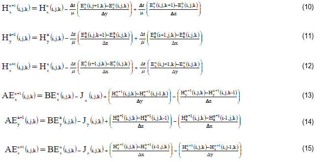
Utilizing the terminology:
Maxwell’s equations, written in component form and applied to the lattice of Figure 2, can be written as shown below:
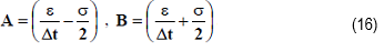
where:
In the above equations, the H-fields exist at times: 0, Δt, 2Δt, 3Δt, … etc., while the E-fields exist at
respective times 1/2 Δt, 3/2 Δt, 5/2 Δt, … etc.
Therefore an Hx-field at time, 3 Δt, is derived from the same Hx-field at time, 2 Δt, neighboring Ez-fields at time, 5/2 Δt,
and neighboring Ey-fields at time 5/2 Δt.
The superscript, “n”, therefore, denotes the time index. In this manner, a marching-in-time algorithm is implemented resulting
in the computation of all electric and magnetic fields at each point in the spatial lattice at particular times.
Since the above equations solve the electromagnetic problem by marching through discrete time steps, the terminology of
“advance equations” is usually applied and will be used in this manual.
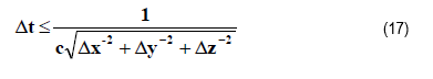
The quantity, Δt, in the advance equations, is referred to as the time increment or finite difference time
step. The time step can be made as small as desired. However, there are limits on the upper value of Δt
that is given by the following equation:
where c is the speed of light in the medium in which the advance equations are being computed.
This condition is known as the
Courant criterion or
Courant condition.
Violation of the Courant condition will result in a numerical instability that is quickly manifested by numerical overflows or the calculation of quantities symbolized
by “Nan” (Not a number). As the equation indicates, the time step can be made as small as desired without violating the Courant condition.
However, a small time step means more time iterations to attain the desired solution.
A consequence of the advance equations is that all H-field components at a particular time, and all E-field
components at a particular time, must be stored in computer memory. There are six (three electric and three magnetic) field components
associated with each finite difference cell. Therefore, the total number of fields, Nfields, within a finite difference computation is:
Nfield = 6(mx)(my)(mz)
where:
mx is the number of cells in the x-coordinate direction
my is the number of cells in the y-coordinate direction,
mz is the number of cells in the z-coordinate direction.
The above equation implies a limited number of cells in each coordinate direction. Electromagnetic problems, however,
are generally unbounded spatially and therefore the region in which field computations are required can be quite extensive.
Exceptions are problems confined to a metallic or PEC enclosure where field values external to the enclosure are considered
negligible. An extensive region of discrete field computations would require prohibitive computer resources.
To circumvent this difficulty, the finite difference lattice must be of limited spatial extent and thus terminated at some
point. If the lattice is terminated, then inspection of Figure 3 and the advance equations, reveal a problem with field
computations on the lattice boundary. To advance these boundary fields requires field components external to the boundary.
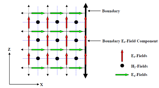
This is illustrated by the two-dimensional depiction in Figure 4.
Assume the lattice is truncated, as indicated in the figure, at the labeled boundary Ez-field component
location. This field component is on and parallel to the boundary. All field components on the boundary,
including this particular Ez-field, are called boundary fields. There are Ey-fields that also share the same
boundary as this Ez-field. The blue dotted lines in the figure indicate the dependencies in the field
component advance equations. The H-field components are thus advanced using the four surrounding electric
field components, one of which may be a boundary field. To advance the boundary Ez-field component would
require an Hy-field outside the boundary, that is not available. Thus, the boundary fields cannot be computed
using the normal advance equations. This is true irrespective of whether the boundary fields are electric or magnetic.