Finite Difference Problem Space

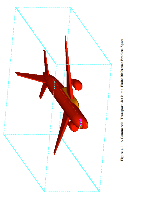
The concept of the finite difference problem space was introduced in the previous chapter. A view of a commercial transport jet within a finite difference problem space in shown in Figure 4.1.1. The finite difference mesh increments can be observed on the cyan border lines. These mesh increments are constant. That is, the mesh increments are uniform along a single coordinate direction. If the mesh increments are the same in all three coordinate directions, then the mesh is cubic. ,

The aircraft within the problem space is immersed within a background medium. For most situations, the background medium is a vacuum. The concept of background media refers to volumes of the problem space to which material properties are assigned that are not explicitly meshed, but are implicitly meshed within EMA3D. In most cases, there is only one background consisting of air or a vacuum. Within EMA3D® a vacuum background is automatically assumed unless defined otherwise. However, there can be multiple background specifications in EMA3D. A background can be specified as linear or nonlinear. All linear backgrounds consist of frequency independent, isotropic material definitions. Nonlinear backgrounds employ a three-species air chemistry formalism for modeling air breakdown and ionization. A nonlinear background is useful when modeling electric discharges in air.

As discussed in the previous chapter, the problem space must be terminated in a boundary condition. There are ten boundary condition types available in EMA3D. The type of boundary condition employed depends upon the problem being addressed. For instance, if electromagnetic responses inside of a metallic enclosure are desired, then perhaps a PEC boundary might be employed. If a symmetry exists, at least in one direction, then perhaps a symmetric boundary might be employed on the necessary boundary. If electromagnetic responses in open air are desired, then a radiating boundary would be employed.

Geometric object may touch or extend beyond the lattice boundary of the finite difference problem space. When employing certain boundary conditions, such protrusions are computationally analogous to extending that part of the intersecting geometry, with the boundary, to infinity and attaching such an extension to the structure within the problem space, as depicted in Figure 4.1.2. This type of configuration is useful if it is determined that the structure outside of the problem space, insignificantly impacts the electromagnetic behavior of that within. Such would be the case for high frequency responses on small sections of a larger structure. These extensions to infinity also allows a large reservoir of charge, or a ground, to drain charge away from an object.