Space Step

The space steps keyword is used to define the mesh increments. There are three different mesh types that can be specified for EMA3D®. These are listed below.

• Constant mesh

• Variable mesh

• Mixed mesh

A constant mesh is one where the spatial increment values Δx, Δy, and Δz are constant and fixed throughout the finite difference problem space. A variable mesh is one where the spatial increment values can vary throughout the problem space. A mixed mesh is one containing both constant and variable mesh increments.

There are several factors that require careful consideration when specifying a finite difference mesh. Discussions of general lattice concepts are discussed below followed by topics exclusive to a three-dimensional configuration and topics exclusive to a two-dimensional configuration.

A constant or uniform mesh is one where the spatial increment values, Δx, Δy, and Δz are constant and fixed throughout the finite difference problem space. These values may not be equal, but are fixed. If the values are equal, then a cubic mesh is defined.

There should be at least ten mesh increments (cells) to resolve the highest frequency, or smallest wavelength, of interest. There is thus an upper limit on the cell size for any frequency band. A higher bandwidth requires smaller spatial increments resulting in larger, and usually more complex, models, thereby requiring more computer memory for execution. The ten required increments pertain to the largest mesh cell dimensions defined by the lattice. Thus, if

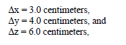
then ten, Δz increments, would be required to resolve the highest frequency of interest. Failure to adequately resolve the higher frequencies results in electromagnetic wave dispersion that impacts the accuracy of computational results. A cubic mesh is thus desirable, from a frequency resolution perspective, because all frequency components propagate equally in all three directions. However, if all frequencies are adequately resolved in all directions, then a noncubic mesh can provide an accurate solution.

The frequencies present within a finite difference problem are created by electromagnetic sources. These sources are discussed in Section 5.6. Electromagnetic sources can be defined to contain negligible frequency content above a particular frequency value. However, many sources such as those defined by various military, commercial, or industrial standards can contain content beyond the interests of the immediate application. Failure to resolve these higher components may result in the initial appearance of numerical noise – although if the content is small, the noise will be minimal.

An isometric view of a commercial aircraft within a finite difference lattice was shown in Figure 4.1. The individual tick marks on the lattice boundary show the spatial increments along the three coordinate directions. The mesh associated with this lattice consists of uniform cubic cells. The spatial extent of the lattice constitutes the finite difference problem space. The number of spatial increments dictates the size of the model. The number of spatial increments associated with the lattice in Figure 4.1 consists of:

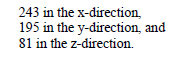
This constitutes a model size of 92 Megabytes for single precision applications.

The size of the problem space is affected by the location of the boundaries. The boundaries in Figure 4.1 are 7 cells from the wing tips. The proper location, or distance from the object being modeled, to define the boundaries depends upon the finite difference boundary condition used. There are many boundary conditions designed for use in different situations. The advantages and disadvantages of each are discussed in Section 5.5.

A variable mesh is one where the spatial increment values, Δx, Δy, and Δz can vary throughout the problem space. A mixed mesh is one containing constant and variable mesh increments. For instance, Δx could possess the values of:

in a problem space containing 22 mesh increments in the x-coordinate direction.

The finite difference spatial lattice of EMA3D can contain any combination of constant or variable mesh sizes in any of the three coordinate directions. For example, a possible lattice definition might result in the following mesh increments.

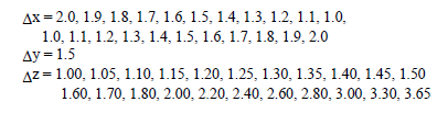
Here the x-increment is variable and decreases from 2.0 down to 1.0, and then increases from 1.0 back to 2.0. The y-increment is constant and set to the value of 1.5. The z-increment is variable and increases from 1.00 to 3.65. The mesh thus consists of 22 x-increments, an unspecified number of y-increments, and 22 z-increments.

A variable mesh can be advantageous in some situations. Parts of the model can be resolved more finely without a significant impact on computer resources. In addition, problem space boundaries can be placed at greater distances by increasing mesh sizes towards the boundary. It is important, however, to understand the ramifications of implementing a variable mesh. The electromagnetic responses computed with such a model possess a higher degree of numerical noise. This is partially a result of the inability of the more coarse mesh increments to propagate the higher frequency components. These components are both dispersed within the coarse mesh and partially reflected by the coarse mesh back towards the more finely meshed regions. To reduce this effect, the electromagnetic source should not possess frequency components that violate the ten-mesh cell requirement, applied to the most coarse mesh increments.

To further reduce the noise, it is recommended that the size difference from one mesh increment value to the next, not change by more than ten percent. For instance, the following consecutive mesh increment:

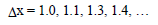
is not recommended, because the x-increment value of 1.3 is greater than the previous value of 1.1 by more than ten percent of the value of 1.1.

When generating the EMA3D input file all lattice index values in a coordinate direction, run from an initial value of 1 to some final value, N, with all meshed objects defined between these bounds. Thus, all lattice indices have positive integral values. For the most part, this is acceptable and transparent to the user. However, it may be necessary to increase the size of the problem space. This could be due to boundary condition effects or perhaps to record additional output information. There are two methods for accomplishing such an increase. The first method involves redefining the spatial lattice within the EMA3D GUI and then remeshing, thus recreating the EMA3D input file. The second step involves editing the existing input file and making appropriate modifications.

The presence of negative indices is allowable in EMA3D. Therefore, if an increase in problem space size on the lower and upper boundaries by an amount equal to, m, was desired, then one could merely change the problem space bounds, 1 and N, in the input file, to values obtained by the operations, 1-m and N+m.