2D Geometries

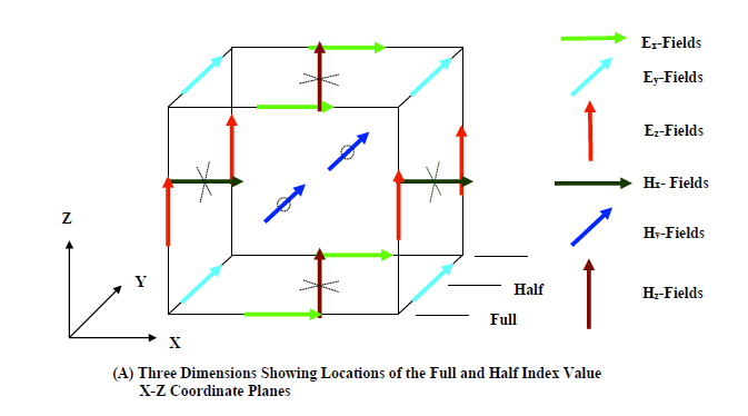
The finite difference technique can also be applied in two dimensions. A two-dimensional description is justified when, in certain regions, two-dimensional behavior closely resembles that of three dimensions. An example may be the high frequency electromagnetic behavior of the center regions of an aircraft fuselage when driven by a plane wave configured for broadside illumination. The finite difference field component configuration for three dimensions is depicted in Figure 3.2.1A. The different components are color coded for clarity. Full and half index planes are also indicated.

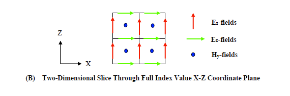
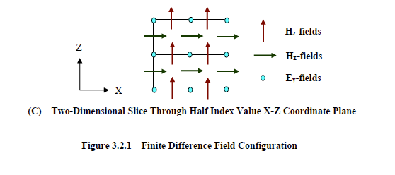
A two-dimensional slice through a full index x-z coordinate plane is shown in Figure 3.2.1B. The corresponding field configuration at a half index x-z coordinate plane is shown in Figure 3.2.1C. The three-dimensional advance equations here, when applied to the two-dimensional lattice of Figure 3.2.1B, reduce to the following three simple equations.

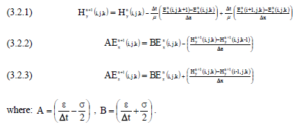
Inspection of these equations reveal less fields and less required computations. Furthermore, the j index is superfluous reducing the amount of memory required by each field. A two-dimensional slice through an existing three-dimensional model, therefore, executes substantially more quickly with significantly less memory. This allows a quick observation and assessment of late time behavior. A two-dimensional model could possibly compute thousands of times faster than the corresponding three-dimensional counterpart. For a given amount of computer memory, a two-dimensional model can be meshed at significantly finer resolutions allowing an accuracy assessment of certain aspects of the corresponding, more coarse, three-dimensional model. The memory required by the above twodimensional configuration is:

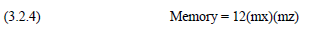
where mx is the number of cells in the x-coordinate direction, and mz is the number of cells in the z-coordinate direction.

A cubic three-dimensional finite difference problem space consisting of 275 cells in each coordinate direction requires 500 megabytes of computer memory. For the two-dimensional x-z plane geometry of Figure 3.2.1B, 500 megabytes would imply a square problem space of dimension 6400. The twodimensional model resolution can be substantially finer than the three-dimensional counterpart.