Transmission Line Finite Difference Formalism |
Equations (3.1) and (3.2) of the previous section can be put in finite difference form. Doing so renders the corresponding equations below:
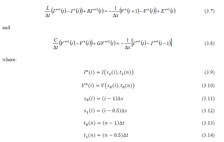
Equation (3.7) and Equation (3.8) can be rewritten as:
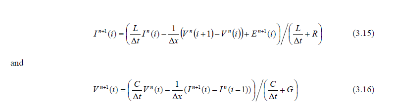
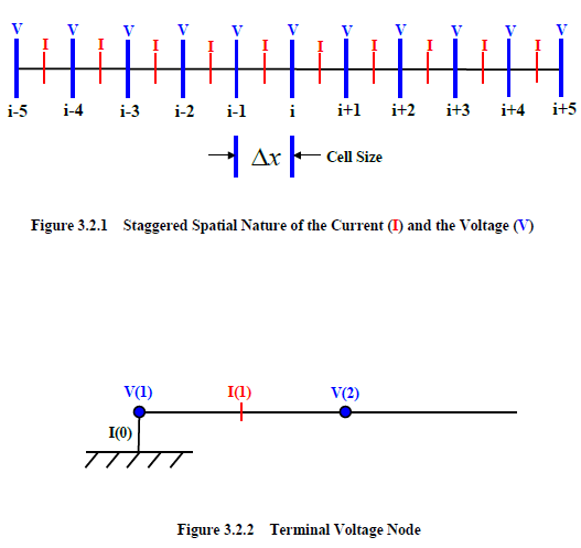
Equation (3.15) and Equation (3.16) are known as the current and voltage time advance equations, respectively, or just the advance equations. A forward differencing scheme is applied to the R and G terms to handle all values of the coefficients. Examination of these equations reveals the staggered nature, in both space and time, of the current and the voltage advance equations. The staggered spatial nature of both the voltage and the current is portrayed in Figure 3.2.1. The spatial increment or cell size is also shown. Examination of the figure reveals the voltages to lie at whole integral index points, or nodes, and the currents at half-integral index points. A special case exists at the end of the line. The line is usually terminated on a voltage node. Examination of Figure 3.2.1 reveals the absence of a necessary current value at either end of the line. For example, if the line began at the index of 1, then the voltage advance equation would be:
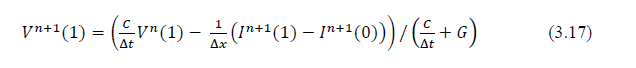
However, there is no I(0) finite difference current available. For this value, the current to ground is used, as shown in Figure 3.2.2. Generally, this current is a function of V(1) and the manner in which the conductors in the line are terminated (that is, the impedance to ground).
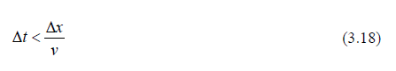
To ensure numerical stability, the cell size must satisfy the Courant condition:
The generalization of Equations (3.15) and (3.16) to the matrix Equations (3.4) and (3.5) is realized by replacing the scalar variables by the corresponding matrices and column vectors.
EMA3D - © 2026 EMA, Inc. Unauthorized use, distribution, or duplication is prohibited.