Surface, Internal, and Coupled Simulations

An example meshed human-space capsule in a worse-case GEO environment to exemplify the fine details of the simulation results.

The surface charging module is based on the boundary element method. In this approach, normal electric fields and potentials on elements are written in terms of the charge density on other surface elements using the superposition principle. Then, matrix relationships can be established between the normal electric field and potentials and a time dependent matrix charging equation can be obtained. A Gaussian-elimination-based algorithm solves the full matrix equation for surface charging (direct solver).

To solve the solutions to the matrix equation, multiple methods can be selected depending on applications:

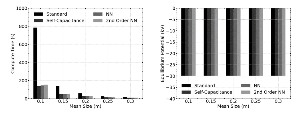
• Standard method – the full matrix solution which approximately grows with the square of the number of surface elements.

• Self-capacitance method – the capacitance with respect to the chassis is calculated for each mesh element and used to solve the charge balance equation.

• Nearest-Neighbor (NN) approximation – approximation to the standard method using sparse matrices to efficiently reach a solution. Additional time for the charge propagation across the surface of the model must be considered. This method provides very accurate results of surface potentials in a steady state by considering the self-capacitance method and that of the nearest neighbors to solve the charge balance equation.

• Iterative solver – alternative algorithm to the direct solver to improve time-to-solution.

• Second nearest-neighbor approximation – default algorithm which is a second order approximation of the NN approximation. This algorithm also has access to an iterative solver for faster time to solution.

Because of the availability of these methods, EMA3D Charge does not limit the resolution of the surface mesh. However, if the problem statement requires detailed simulation of the charge propagation along the material surface, then the standard method is the go-to method.

Compute time and simulated equilibrium potential for a 1-m aluminum CubeSat with 2 opposing Kapton faces, in a worse-case GEO environment for 100 seconds at 100 time steps.

The surface charging is driven by various current sources: environmental driven current density from either Maxwellian or Kappa distributions, including the secondary electron yields, backscattered electron yields, and proton induced electron yields, photoemission from sunlight illumination, currents due to surface and volume conduction, triboelectrification, and currents from particle transport include plume and other high energy particle sources. More about sources will be described later in this section.

The physics equations behind each contribution are described in the technical section of this manual.

An example meshed dielectric slab with a screw demonstrating the resolution of the mesh and the simulated enhanced fields at the tip. The projection of the internal mesh elements, as well as the surface mesh elements are visible.

The internal charging module is based on EMA’s quasi-static electrodynamics finite element method (FEM) coupled to a particle transport source. In this approach, at each time step charge density from the particle transport is evaluated in each finite element volume to obtain a source term for the finite element matrix equation. There is great generality in the types of internal charging environments that can be specified. The finite element solver uses the Biconjugate gradient stabilized method (with an option for higher order polynomials) to solve the matrix equations.

The 3D particle transport source is coupled to the FEM such that the charge deposited by parent and daughter particles during interactions is changing the local conductivity of the material and the electric fields. Those fields are then coupled back to the particle transport tool as they affect the subsequent interaction processes.

The FEM also includes a particle-in-cell (PIC) code to manage the effect of the electromagnetic field, generated by surface charging, on the surrounding plasma environment. The charged particle density and flux is tracked from one volumetric cell to another and the simulations account for their contribution to the charge balance equations.

To tackle complex charging environments that combine the effects of low energy plasma with the effects of high-energy particle, surface charging and internal charging may be combined in a variety of ways. Surface potentials obtained from surface charging may be used as boundary conditions in the internal charging simulations, updated on per time step basis. Current flux from the particle transport environments may also be included in the surface charging simulations, typically incorporated up to some threshold energy value. In this way, there is a dynamic integration of surface charging and internal charging physics.

Ultimately, by coupling the surface charging module to the FEM, and the particle transport source of the internal charging module, EMA3D Charge handles the following space-related charging environments:

• GEO – surface charge balance

• Lunar – surface charge balance

• LEO – surface charge balance, FEM, particle-in-cell code

• Auroral – surface charge balance, FEM, particle-in-cell code

• Solar Wind – surface charge balance, FEM, 3D particle transport

• Plasma Sheet – surface charge balance, FEM, particle-in-cell code

• Plumes - surface charge balance, FEM, particle-in-cell code, 3D particle transport

The particle-in-cell code will be available Q4 of 2021.